Download
1 / 57
570 likes | 634 Views
Labs for course #412 Analyzing Microarray Data using the mAdb System July 15-16 , 2008 1:00pm- 4:00pm. First, look at the questions on the bottom of each page. Write down the answers while going through the steps on the page.

E N D
Labs for course #412Analyzing Microarray Data using the mAdb SystemJuly 15-16, 2008 1:00pm- 4:00pm • First, look at the questions on the bottom of each page. Write down the answers while going through the steps on the page. • Keep the browser NOT maximized so multiple windows can be distinguished.
Lab 1. Copying a Training Dataset Goal: To copy a dataset into user’s temporary area and to inspect dataset features.
4 Lab 1. Copying a Training Dataset 1. Open a web browser and type the URL for the mAdb home page, for training class: http://madb-training.cit.nih.gov -use login on name tent and password on board. Others can use http://madb.nci.nih.gov (NIAID users http://madb.niaid.nih.gov) and log in with your mAdb account. 2. Click the mAdb Gateway link to access mAdb Gateway Web page 3. On the mAdb Gateway Web page, click the link Access Training/Public Dataset on the bottom of the page. A page for copying three training datasets will be presented. 4. You can choose to work with either "Small, Round Blue Cell Tumors (SRBCT) dataset" or "NEJM Dataset". Click link Copy to copy the dataset into your temporary area. 5. After copying the data, you will see the temporary dataset area. Click link Open on the selected dataset line.A mAdb Dataset Display page will be displayed. 5 Questions: 1. How many genes and how many arrays do you have in your dataset?
1 1. On the mAdb Dataset Display page, review the title bar, or the dataset description on top of the page. This tells you which dataset you are displaying. 2. In the Dataset Retrieval & Display Options panel, check the Show Array Details at the top of the page option. Then click Redisplay button. The names and short descriptions of arrays in the dataset will be displayed on the top of the page. Look for naming conventions of the array and then answer the question below. This information will be used in the next lab. After reviewing the array details, it is recommended to uncheck the Show Array Details at the top of the page option. Click Redisplay to hide the array details on the top of the page. 3. Check or uncheck other display options of interest, and click Redisplay button to display or hide the relevant information. Uncheck Show Data Values and set Background Color to None will make it easier to view other annotations. 2 3 Questions: 1. How many experiment groups can you identify in this dataset by their naming conventions? Write down the naming conventions for each group. Lab 1. Copying a Training Dataset
Lab 2. Assigning Group Labels Goal: To partition arrays into groups according to experiment design by assigning group labels.
2 1 Lab 2. Assigning Group Labels 3 In the Filtering/Grouping/Analysis section, choose the Filter/Group by Array Properties Tool 2. Click on Proceed A new page will be displayed with options for assigning arrays into groups by the naming convention of Array Name or Short Description. 3.For the SRBC dataset, use EWS, BL, NB, RMS as matching patterns. Select Array Name and Begins with from the drop down list for each group. Samples with name beginning with "Test" are excluded from the grouped subset. For the NEJM dataset, use GCB, ABC, and Type as matching patterns. Select Array Name and Begins with from the drop down list for each group. 4. The grouped results are stored as a new subset. Enter an appropriate label for this subset. 5. Click on Submit. There is no “Waiting” page, the new grouped subset will be directly displayed when the Group/Filtering process is completed. 4 5
Lab 2. Assigning Group Labels 1 Examine the grouped subset through the dataset description and history on top of the Dataset Display page. Questions: • How many arrays are filtered out in the grouped dataset? • What are they? Hint use “Array Order Designation/Filtering Tool”. • How many arrays do you have in each group? Write down the group designations for each tumor type.
Lab 3. Generating a Correlation Summary Report Goal: To study the correlation of expression data among samples in the dataset.
3 2 Lab 3. Generating a Correlation Summary Report • Verify that the current dataset is My Grouped Dataset through title bar or dataset description. (See Lab 1, Dataset display section for details) • 2. In the Filtering/Grouping/Analysis section, choose the Correlation Summary Report Tool. (You may have to scroll down the Tool dropdown list to find it on the bottom.) • 3. Click on Proceed. • mAdb Correlation Report page will be displayed with a table of correlation results. • 4. Change the Background Color Scheme to Green/White/Red. • 5. Inspect the values of the correlation tables and set the values for Color Saturation. For SRBCT dataset, use 0.8, 0.6, 0.4. For NEJM-3 class dataset use 0.3, 0.0, -0.3. • 6. Click on Redisplay button. Correlation table will be colored according to the correlations. 4 5 6
Lab 3. Generating a Correlation Summary Report 2 3 • The image shows part of the correlation table. The color pattern uses green for good correlations and red for poor correlations. • Each correlation number represent a pair-wise correlation calculation between 2 samples. It can be clicked to display a scatter plot between the 2 samples. Click on a larger number to display the scatter plot for 2 correlated samples. • Click a small number to display a scatter plot for 2 poorly correlated samples . • Questions: 1. Describe the general color pattern of the correlation table. Are correlation numbers within a group better(more green) than between groups(more red)? 2. How is the scatter plot of a good correlation different from a plot of a poor correlation?
Lab 4. Filtering Data Goal: To pre-process a dataset for further analysis by filtering out genes with low variance or with many missing values.
3 2 Lab 4. Filtering Data • Use back button on web browser to return to previous Dataset Display page. Verify that the current dataset is My Grouped Dataset. (See Lab 1, Dataset display section for details). • In the Filtering/Grouping/Analysis section, choose the Additional Filtering Options Tool. • Click on Proceed • Data Filtering Options page will be displayed with options for Missing Value Filters and Gene Filters. Be careful to check the "checkboxes" along putting in values in step 4-9. • Select the check box for Genes: Require values in >= • Set the value to 95% of arrays. • Select the check box for Variance (Gene Vector) percentile • Set the value >= 90% • The filtered results are stored as a new data subset. Enter an appropriate Label for this subset. • Click on Filter. Filtering will be performed and the results stored as a new subset. There is no “Waiting” page, the new subset will be directly displayed when the Filtering process is completed. 5 4 7 6 8 9
Lab 4. Filtering Data 1 1. Review the subset history on top of the Dataset Display page for the filtering. 2. Click link History, a new window will popup with the full dataset history. Review the text. 3. Click output Dataset will lead you to the filtered dataset. Close the new window and return to the previous window. 2 3 Questions: 1. How many genes are filtered out by missing values? How many genes are filtered out by variance?
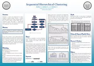
Lab 5. Hierarchical Clustering Goal: To cluster genes and/or arrays with the Hierarchical Clustering algorithm.
2 1 Lab 5. Hierarchical Clustering Verify that the current dataset is the filtered dataset. (Gene>=95, Variance>=90) • In the Filtering/Grouping/Analysis section, choose the Clustering: Hierarchical Tool. • Click on Proceed • A new page will be displayed with options for selecting the Similarity/Distance Metric. • Choose Correlation (centered classical Pearson) to cluster both Genes and Arrays. • Click on Cluster button. 3 4
Lab 5. Hierarchical Clustering 1 A new page will be displayed for Hierarchical Clustering progress. When the analysis is done, a View Clusters button is displayed on top of the page. • Click the View Clusters button at the top of the page or the Click to view result link at the bottom. • A new page will be displayed with a thumbnail image of the clustering results
Lab 5. Hierarchical Clustering 1 Click the thumbnail on the page. • A new browser window will open up to display a enlarged heatmap image, gene trees and array trees. • Check the array tree structure. Check the relationship among all the tumor groups. • The color bar indicate the grouping information of arrays. Identify the misclassified samples. Speculate possible explanations. • Click on the gene annotations on the right. A new window will open up with a feature report page. Close the Feature Report window. Close the Heatmap display window. Return to the thumbnail image window. 2 3 4 Questions: 1. How do the tumor samples cluster together? Can you find duplicate genes that cluster together on the heatmap?
Lab 6. SOM Clustering Goal: To partition genes into a 2-dimensional topology using the Self Organizing Map (SOM) algorithm and to observe genes with similar expression patterns.
3 2 Lab 6. SOM Clustering Use the back button of the browser to return to the previous Dataset Display page. Verify that the current dataset is the right dataset. (Gene>=95, Variance>=90) 2. In the Filtering/Grouping/Analysis section, choose the Clustering: SOM Tool 3. Click on Proceed A new page will be displayed with options for SOM. 4. Select Median Center Genes before Clustering 5. Set X dimension to be 4 and Y dimension to be 3, number of iterations to be 100000. Uncheck the checkbox for Initialize with Randomized Partition. 6. Set the Hierarchical Clustering Options within the SOM clusters. Select Correlation (centered –classical Pearson) Metric for Genes and Not Clustered for arrays. 7. Click on Cluster button. A new page will be displayed for SOM Clustering progress. When the analysis is done, a View Clusters button is displayed on top of the page. 8. Click the View Clusters button. A new page will be displayed with a thumbnail image of the clustering results 4 5 6 7
Lab 6. SOM Clustering 2 1. Inspect the spatial relationship among the clusters. 2. Click a thumbnail image on the page. A new browser window will open up to display an enlarged heatmap image and gene tree of the clicked thumbnail image. 3. Note similar genes and compare expression results. 4. Click on Line Plot View 3
Lab 6. SOM Clustering 2 1. Inspect the spatial relationship among the clusters. 2. Click a thumbnail image on the page. A new browser window will open up to display an enlarged line plot image and gene tree of the clicked thumbnail image. 3. Can you interpret the graph? Questions: 1. Do genes in the same partition show a similar expression profile? How are the expression profiles different among different partitions (2-D topology)?
Lab 7. K-means Clustering (Optional) Goal: To partition genes into K numbers of partitions using the K-means algorithm and observe genes with similar expression patterns.
Lab 7. K-means Clustering 2 1. Use the back button of the browser to return to the previous Dataset Display page. Verify that the current dataset is the right dataset. (Gene>=95, Variance>=90) 2. Click link Expand this Dataset above the Filtering/Grouping/Analysis Tools section. You will then be presented an expanded dataset selection page. You will find the dataset and all the subsets you saved from previous analysis. 3. Click link Open open My Grouped Dataset. A mAdb dataset display page will be presented to you. K-means clustering will be performed on the full grouped dataset to show its performance speed advantage. 3
1 2 Lab 7. K-means Clustering 1. In the Filtering/Grouping/Analysis section, choose the Clustering: Kmeans Tool. 2. Click on Proceed. A new page will be displayed with options for Kmeans Clustering. 3. Select Median Center Genes before Clustering 4.Specify Number of Nodes to be 12. Set Maximum Number of iterations to be 100. 5. Set the Hierarchical Clustering Options within Kmeans Nodes. Select Correlation (centered –classical Pearson) for Genes and Not Clustered for arrays. 6. Click on Cluster button. A new page will be displayed for Kmeans Clustering progress. When the analysis is done, a View Clusters button is displayed on top of the page. 7. Click the View Clusters button. A new page will be displayed with a thumbnail image of the clustering results. 3 4 5 6
2 Lab 7. K-means Clustering 1. Inspect the thumbnail images for the expression patterns within the clusters (Only 6 out of 12 clusters are displayed here). 2. Click thumbnails of interest on the page. A new browser window will open up to display an enlarged heatmap image and gene tree (not shown here) of the clicked thumbnail image. 3. Close the Heatmap display window. Return to the thumbnail image window. Questions: • Are the expression profiles different among different partitions? • Can you interpret the expression profile of a given gene?
Lab 8. PCA Goal: To explore the data structure of the dataset using Principal Component Analysis (PCA).
Lab 8. PCA 2 3 1. Verify that the current dataset is the filtered dataset. (Gene>=95, Variance>=90) 2. In the Interactive Graphical Viewers section, choose the viewer, PCA: Principal Components Analysis. 3. Click on View button. A new window, PCA Options, will be displayed with options for the PCA Analysis . 4. Select to perform PCA on Arrays. 5. Select Dispersion Matrix of Covariance. 6. Click Continue button. A new page, Waiting for PCA, will be displayed. When PCA analysis is done, a summary and a new button, 3D Viewer will be displayed on the page. 7. Click 3D Viewer button. • Questions: • 1. How many genes are used in PCA analysis? (Genes with missing values are not used in PCA) 4 5 6 7
1 Lab 8. PCA 1. Check the percentage of Variance represented in the 3D plot. Does it capture a large percentage of total variance? 2. Click the X, Y and Z buttons to rotate the 3-D plot. Look for clustering /separation of data. Click Stop button. 3. Click and Drag the mouse to highlight an area of the 3 D plot. Data points in the area will be displayed in the text area below the plot. 4. Click the link Details on the bottom of the 3D viewer. A new page, PCA details, will be displayed with 4 additional plots from PCA analysis. See next page for more description of the PCA details page. Questions: 1. What is the percentage of variance represented in the first three components? 2. What is the color-coding for each group of samples? Can you see a separation of different groups in 3D plot? 3 2 4 5
Lab 8. PCA 1 3 1. The Scree Plot displays the Variance for individual components. Click on the plot will display a new page with an enlarged image. 2. The PDF (Portable Document Format) or PNG (Portable Network Graphics) links under each figure can be used to display or save a larger image of the figure. You can also save a larger image as Encapsulated PostScript using the EPS link 3. The other three plots shown are 2-D plots for each combination of the first 3 components. 4. The Retrieve button will retrieve the data back to your local computer. Several options are available. We do not need to retrieve data for this Lab. 5. Click the link Click to Close to close the viewer. This will allow you to go back to the starting dataset display page. Questions: 1. In the scree plot, identify where the slope of variance flattens out (the scree point). 2 4 5
Labs for course #412Analyzing Microarray Data using the mAdb SystemJuly 15-16, 2008 1:00pm- 4:00pm • First, look at the questions on the bottom of each page. Write down the answers while going through the steps on the page. • Keep the browser NOT maximized so multiple windows can be distinguished. Day 2
Lab 9. Performing an ANOVA analysis Goal: To identify differentially expressed genes using class comparison statistical tools.
Lab 9. Performing an ANOVA analysis 1 • On the mAdb Gateway Page, Click on Temporary area to open a list of your Datasets stored in this area. • Click on the Expand for the “Small Round Blue Cell Tumors (SRBCTs)…” (or, if you are using the other dataset, Expand for the “NEJM – 3 Classes”) to open the list of Subsets for this Dataset. • Click on the Open for the “My Grouped Dataset” subset. 2 3
1 2 Lab 9. Performing an ANOVA analysis • In the Filtering/Grouping/Analysis section, choose the Group Comparison Tool • Click on Proceed A new page will be displayed with options for the statistical comparison analysis. Since this dataset has more than two groups, only the Multiple Group Comparison options for more than two groups will be available for selection. • Select One way ANOVA • Analysis results are stored as a new subset. Enter an appropriate Label for this subset. • Click on Proceed. 3 4 5
Lab 9. Performing an ANOVA analysis A “Waiting” page is displayed while the analysis is being performed. When the analysis is completed, the continue button is displayed. • Click on Continue. A mAdb Dataset Display page, displaying the newly created subset which contains the ANOVA analysis results will appear. 1 The three columns, p-Value, Difference and Groups display results from this analysis.The p-Value is the One way ANOVA calculation. The Difference displays the largest difference between group means--this calculation is independent of the ANOVA calculation. The Groups identifies the two groups having this largest mean difference. The default order of the data is from smallest to largest p-Value. Note that “Show Data Values” has been unchecked for the display shown here.
1 2 Lab 9. Performing an ANOVA analysis • In the Filtering/Grouping/Analysis section, choose the Statistical Results Filtering Tool • Click on Proceed A new page will be displayed with the options for filtering the statistical results. • Check the box to the left of One way ANOVA p-value, select “<=“ and enter the p-value as 0.000001 or 1e-7. • The filtered results will be stored as a new subset. Enter an appropriate Label for this subset. • Click on Filter. Filtering will be performed and the results stored as a new subset. There is no intermediate “Waiting” page, the new subset will be directly displayed when the Filtering process is completed. 3 4 5 Questions: 1. How many genes are there in the filtered dataset?
In order to facilitate later comparison/filtering of these results with other results, we will save this result as a Feature Property List. Lab 9. Performing an ANOVA analysis 1 • Click on Save a Feature Property List. A new page will be displayed with the options for the Saving a Feature Property List.. • Select mAdb Well IDS • Select Global (Available in all Datasets) • Enter an appropriate label to identify this List • Click on Save 2 3 4 5
Lab 9. Performing an ANOVA analysis 1 A page indicating that the List was successfully stored and summarizing information about the list will be displayed. 1. Click on Continue. This will return you back to the Data Display Page.
Lab 10. Using SAM Goal: To evaluate statistically significant genes and determine the False Discovery Rate (FDR).
Lab 10. Using SAM 1 • On the mAdb Gateway Page, Click on Temporary area to open a list of your Datasets stored in this area. • Click on the Expand for the “Small Round Blue Cell Tumors (SRBCTs)…” (or, if you are using the other dataset, Expand for the “NEJM – 3 Classes”) to open the list of Subsets for this Dataset. • Click on the Open for the “My Grouped Dataset” subset. 2 3
Lab 10. Using SAM 2 1 • In the Filtering/Grouping/Analysis section, choose the Filter/Group by Array Properties Tool • Click on Proceed A new page will be displayed with options for assigning arrays into groups by the naming convention of Array Name or Short Description. • For the SRBC dataset, use BL and NB as matching patterns. Select Array Name and Begins with from the drop down list for each group. For the NEJM dataset, use GCB and ABC as matching patterns. Select Array Name and Begins with from the drop down list for each group. • The grouped results are stored as a new subset. Enter an appropriate label for this subset. • Click on Submit. There is no “Waiting” page, the new grouped subset will be directly displayed when the Group/Filtering process is completed. 3 4 5
2 1 Lab 10. Using SAM • In the Filtering/Grouping/Analysis section, choose the SAM: Significance Analysis for Microarrays Tool. • Click on Proceed. • Click on SAM help. • Select SAM options to Remove missing values, to perform 500 permutations, and set Yes for a fixed random seed. • Click on Continue. 3 4 5
Lab 10. Using SAM SAM Analysis is initiated and a “waiting” page is displayed. When the Analysis is complete, an analysis summary and a button to continue to the next step appear on the page. 1. Click on SAM Step2. 1 Questions: 1. How many genes contain missing values?
Lab 10. Using SAM The SAM results are displayed as a table and three graphs. The table shows the number of significant genes, the number of false genes and the false discovery rate (FDR) for each Delta. You can create a subset containing the genes corresponding to one of the models by either clicking on a Delta value or entering a Delta value in the text box and clicking the “Create Subset” button. The top left graph plots the Delta vs. the FDR. The top right graph plots the Delta vs. the number of significant genes. The lower graph plots the observed d(i) vs. expected d(i), with a delta cutoff that generates the biggest FDR that is smaller than 0.05. Click on an image icon with a low FDR (new window pops up.) Click on a Delta with a low FDR. Questions: • How many genes do you have for this Delta? • What is the FDR for the Delta? 1 2
Lab 10. Using SAM • A mAdb Dataset Display page, displaying the newly created SAM subset appears. • Note that Show Data Values has been unchecked and the Background Color has been set to None for the display shown here.
Lab 11. Using PAM Goal: To evaluate shrunken centroid prediction models and identify sets of genes that best classify sample types.
Lab 11. Using PAM 1 • On the mAdb Gateway Page, Click on Temporary area to open a list of your Datasets stored in this area. • Click on the Expand for the “Small Round Blue Cell Tumors (SRBCTs)…” (or, if you are using the other dataset, Expand for the “NEJM – 3 Classes”) to open the list of Subsets for this Dataset. • Click on the Open for the “My Grouped Dataset” subset. 2 3
2 1 Lab 11. Using PAM 1. In the Filtering/Grouping/Analysis section, choose the PAM: Prediction Analysis for Microarrays Tool. 2. Click on Proceed PAM Analysis is initiated and A “waiting” page is displayed. When the Analysis is complete, an analysis summary and a button to continue to the next step appears on the page. 3. Click on PAM Step2. Questions: 1. How many fold of Training and Cross Validation was performed? 2. How many genes contain missing values? How many missing values are imputed for the dataset? 3
Lab 11. Using PAM The PAM results are displayed as a table and two graphs. The table shows the Shrinkage Delta (** indicates those having minimum misclassification error), number of genes in the model and the misclassification error based on the K-fold cross validation. You can create a subset containing the genes corresponding to one of the models by either clicking on a Shrinkage Delta value or entering a Delta value in the text box and clicking the “Create Subset” button. The top graph plots the misclassification error (with error bars) versus the Shrinkage Delta (bottom axis) and the number of Genes (top axis). The lower graph plots the misclassification error for each group versus the Shrinkage Delta (bottom axis) and the number of Genes (top axis).
Lab 11. Using PAM • Click on a Shrinkage Delta having a minimum misclassification error. Questions: • How many genes do you have in the model ? • What is the Misclassification Error percentage for the model? 1
Lab 11. Using PAM • A mAdb Dataset Display page, displaying the newly created PAM subset appears. • The columns A Score, B Score, … contain the shrunken differences for each group. Non zero values can be used to infer which group or groups a gene’s expression value distinguishes. • Note that Show Data Values has been unchecked and the Background Color has been set to None for the display shown here.