Download

1 / 111
1.14k likes | 1.5k Views
Scheduling. THE SCHEDULING ACTIVITY AT MACHINE SHOP. Objectives (goals) of Scheduling . As it was previously mentioned, there are three primary objectives (goals) which apply to all scheduling problems: Job completions should not be “late” (about due dates).

E N D
Scheduling THE SCHEDULING ACTIVITY AT MACHINE SHOP
Objectives (goals) of Scheduling • As it was previously mentioned, there are three primary objectives (goals) which apply to all scheduling problems: • Job completions should not be “late” (about due dates). • The the length of time during which a job stays in the system should be “minimum” (about flow time) • It is desired to fully utilize the capacities of work centers (about work center utilization).
Kinds of Scheduling Problems Studies about scheduling activity point out that there are two fundamental kinds of scheduling problems. Dynamic Scheduling Problems Static Scheduling Problems deals with scheduling of a continuous situation, which means that, new jobs are continually added to the production environment. where, problem consists of a fixed set of jobs which are to be all completed. The number of jobs does not change.
Static Scheduling Approach • The static scheduling problem contains a fixed set of jobs which are to be completed. • The typical basic assumptions in this kind of problem can be stated as follows; • ... entire set of jobs arrive simultaneously, and • all respective work centers are available at that time. • Majority of the static scheduling problems use a criterion called “minimum make span” which can be defined as the minimum total time to process all subject jobs. This criterion is related with the scheduling objective which is about “flow time”.
Static Scheduling Approach Static Scheduling Problems Deterministic Solutions Stochastic Solutions use process times which are subject to random variations. use known and nonvarying process times. Methods Utilizing Heuristic Procedures Methods Producing Optimum Results scheduling decisions are made sequentially rather than at once called dispatching or sequencing rules. only applicable to relatively small problems.
Dynamic Scheduling Approach Dynamic Scheduling Problems Deterministic Solutions Stochastic Solutions Analytical approaches had been developed which are “based on queuing models that provide expected steady state conditions for certain kinds of situations and time distributions”. Typically, the criteria used in such queuing cases are; Avarage Flow Time Average Work-in-process or number of jobs in the system and Work/ machine center utilization. To find a solution to dynamic scheduling problems, usually the approach is, to use different “dispatching rules” at the work centers.
Job Shop Dispatching and Common Priority Sequencing Rules At any given point in time, there exists a set of “n” jobs to be scheduled on “m” machines. This means, at any time there are (n!)m possible ways to schedule the jobs.
Job Shop Dispatching and Common Priority Sequencing Rules One method to generate schedules in job shops is with “dispatching” which allows the schedule for a work station to evolve over a period of time. The decision about which job to process next is made with simple priority rules whenever the work station becomes available for further processing. Major advantage of “dispatching” method is that latest information on operating conditions of the work center can be incorporated into the schedule as it evolves.
Job Shop Dispatching and Common Priority Sequencing Rules Common Priority Sequencing Rules MULTIPLEDIMENSIONRULES SINGLE DIMENSIONRULES First Come First Served (FCFS) (single dimension) Slack per Remaining Operations(S/OP) (multiple dimension) Earliest Due Date (EDD) (single dimension) Shortest Processing Time (SPT) (single dimension) Critical Ratio (CR) (multiple dimension)
Job Shop Dispatching and Common Priority Sequencing Rules • They base the priority on single aspect of the job, such as, arrival time, the due date, or the processing time at the current work center. SINGLE DIMENSIONRULES • They incorporate information about the remaining work centers at which the job must be processed, in addition to the processing time at the present work station or the due date considered by single dimension rules. MULTIPLEDIMENSIONRULES
Job Shop Dispatching and Common Priority Sequencing Rules • The critical ratio is calculated by dividing “the time remaining until the due date of the job” by the “remaining total shop time for the job”. • CR = [Due date of the job-Today’s date] / Σ remaining shop time • CR < 1.0 implies that the job is behind schedule, • CR = 1.0 implies that the job is on schedule CR > 1.0 implies that the job is ahead of schedule. • The job with the lowest CR is scheduled next. Critical Ratio (CR) (multiple dimension)
Job Shop Dispatching and Common Priority Sequencing Rules • There may be different ways to set the due dates of jobs. For example, a due date might have been calculated by computerized methods as in MRP or might have been simply determined by the customer. • The job with the earliest due date is the job which is to be scheduled next. Earliest Due Date (EDD) (single dimension)
Job Shop Dispatching and Common Priority Sequencing Rules • The job which arrives the work station earlier than the others has the highest priority and is to be scheduled next. First Come First Served (FCFS) (single dimension)
Job Shop Dispatching and Common Priority Sequencing Rules • Slack is the difference between “the time remaining until the due date of the job” and “remaining total shop time for the job” including that of the operation being scheduled. • The job’s priority is determined by dividing the slack by the number of the operations that remain including the operation which is being scheduled. • S/RO = [(Due date – Today’s date)-Total shop time remaining]/ Number of remaining operations Slack per Remaining Operations(S/OP) (multiple dimension)
Job Shop Dispatching and Common Priority Sequencing Rules • King of the priority sequencing rules! • The job which has the shortest processing time is scheduled next. Shortest Processing Time (SPT) (single dimension)
Job Shop Dispatching and Common Priority Sequencing Rules • There are nalso some other rules most of which can be considered as variants of the already mentioned ones ; • The principle is picking any job in the queue with equal probability. • This rule is often used as a benchmark for other rules. In other words, it is used for evaluation of other rules with respect to each other by using reference values obtained from using R rule. Random (R) (single dimension)
Job Shop Dispatching and Common Priority Sequencing Rules • There are nalso some other rules most of which can be considered as variants of the already mentioned ones ; • It is an extension of SPT rule in the sense that it considers all processing time remaining until the job is completed. • This means that, the next job to be processed is the one which has least work remaining along its routing including the work in current station. Least Work Remaining (LWR) (multiple dimension)
Job Shop Dispatching and Common Priority Sequencing Rules • There are nalso some other rules most of which can be considered as variants of the already mentioned ones ; • This rule is again another variant of SPT rule. It considers the number of successive operations. • The next job to be picked is the one which has smallest number of successive operations including the operation being scheduled. Fewest Operations Remaining (FOR) (multiple dimension)
Job Shop Dispatching and Common Priority Sequencing Rules • There are nalso some other rules most of which can be considered as variants of the already mentioned ones ; • It is a variant of EDD rule. It subtracts “remaining total shop time for the job” including that of the operation being scheduled from the “time remaining until the due date”. The resulting value is called “slack”. • Slack time =(due date - today’s date) - (remaining processing time) • Jobs are run in the order of smallest amount of slack. Slack Time (ST) (multiple dimension)
Job Shop Dispatching and Common Priority Sequencing Rules • There are nalso some other rules most of which can be considered as variants of the already mentioned ones ; • This is a different kind of rule which is based on machine utilization. • It considers the “next queues” at each of the succeeding work centers to which the jobs will go. • It selects the job which is going to the smallest queue. Here, the measure of the queue might be either in hours or perhaps in number of jobs. Next Queue (NQ) (multiple dimension)
Job Shop Dispatching and Common Priority Sequencing Rules • There are nalso some other rules most of which can be considered as variants of the already mentioned ones ; • This is another rule for which the objective is to maximizemachine (capacity) utilization. • It selects the job which has minimum setup time on the machine. • It should be noted that, this rule clearly considers dependencies between setup times and job sequence (setup time for a specific job may change according to sequence). Least Setup (LSU) (single dimension)
Job Shop Dispatching and Common Priority Sequencing Rules • There are nalso some other rules most of which can be considered as variants of the already mentioned ones ; • is the difference between a late job’s due date and its completion time TARDINESS (single dimension)
Job Shop Dispatching and Common Priority Sequencing Rules Altough priority sequencing rules seem to be simple, the actual task of scheduling hundreds of jobs through hundreds of work centers requires intensive data gathering and manipulation. The scheduler needs information on each job’s processing requirements; “the job’s due date”, “its routing”, “the standard setup at each operation”, “the processing time at each op.”, “the expected waiting time at each op”; “whether alternative work centers could be used at each operation”, “the components and raw materials required at each operation”, and “the current status of the job”. Computers are needed to track the data and to maintain valid priorities. Any priority sequencing rule can be used to schedule any number of work centers with the dispatching procedure.
Job 1 Job 2 Job n Machine A Priority sequencing rule Single (One)-Machine Case “single-machine” environment is the simple and special case of all other or more complex environments. Single (One) Machine Case The results of single-machine problems not only provide insight to the single-machine environment, but also, provide a basis for heuristics of more complex environments. In most of the practical applications, scheduling problems in complex environments are broken down into smaller sub problems each of which becomes a single-machine case.
Job 1 Job 2 Job n Machine A Priority sequencing rule Single (One)-Machine Case • Problem Definition for Single-Machine Case • Majority of the studies on single-machine scheduling is based on the static problem of how to best schedule a fix set of jobs through a single machine with the assumptions that; Fixed set of jobs are available at the start of the scheduling period Machine A is available when the fixed set of jobs arrive. setup times are independent of the sequence.
Single (One)-Machine Case • What is meant by saying “setup times are independent of sequence”? • Simply, it means, setup times does not alter the total make-span of the entire set of jobs no matter in which sequence the jobs are processed. • In this case, the total make-span equals the sum of all setup and run times for any sequence of jobs
Single (One)-Machine Case • What is meant by saying “setup times are independent of sequence”? A DRILL MACHINECASE
Single (One)-Machine Case • What is meant by saying “setup times are independent of sequence”? • Where setup times are sequence dependent, the total make-span is altered with a change in sequence of jobs. A FURNACE CASE
Single (One)-Machine Case • What is meant by saying “setup times are independent of sequence”? • As a result one may come up with the conclusion that development of analytical models for the case of single-machine problems where setup is sequence dependent is rather complex. • In this respect, it is fortunate that, in most of the single-machine environments make-span does not depend on the sequence (sequence independent).
Application of Single-Dimension Rules (Analysis of Single-Machine Case where setup times are independent of sequence) • If theobjective isto “minimizethemake-span” (minimize the total time to run the entire set of jobs), it is clear that make-span will be equal to sum of all “setup+run” times andwill be same for all sequencing options. • However, if theobjective isto “minimize the average time each job spends at the machine”, it can be shown that this can be achieved by sequencing jobs in ascending order according to their total processing time (setup+run time).
Application of Single-Dimension Rules (Analysis of Single-Machine Case where setup times are independent of sequence) • We can show this fact by the following example : Average Flow Time = Sum of flow times / Number of jobs where, Sum of Flow Times = Σ [waiting time+(setup time+processing time)] values for each job in the system
Application of Single-Dimension Rules (Analysis of Single-Machine Case where setup times are independent of sequence) • In this example : “average time in the system” The Criterion was ... “minimize the average time each job spends at the machine”, The Objective was ... The Rule used was ... SPT Average Flow Time = Sum of flow times / Number of jobs The Measure used was ... The average time in the system will always be minimized by processing the next job which has the shortest processing time at the current operation.
Application of Single-Dimension Rules (Analysis of Single-Machine Case where setup times are independent of sequence) • SPT also proves to be very usefull when the objective is “minimizing the average number of jobs in the system” in a single-machine case. • This time, the measure which we are going to use is “average work-in-process (wip) inventory” for which the formulation is; Avarage wip inventory = Sum of flow times / Make-span
Application of Single-Dimension Rules (Analysis of Single-Machine Case where setup times are independent of sequence) • Example :
Application of Single-Dimension Rules (Analysis of Single-Machine Case where setup times are independent of sequence) • Here, at this point, we should also note that “average wip inventory” and “average flow time” measures are directly related with each other. That is, when the value of one decreases, the value of the other also decreases and vice versa. • Compare the results in previous example and following example.
Application of Single-Dimension Rules (Analysis of Single-Machine Case where setup times are independent of sequence) • Example :
Application of Single-Dimension Rules (Analysis of Single-Machine Case where setup times are independent of sequence) • When the objective is to “minimize the average job lateness”, again SPT seems to yield better overall results in sequencing jobs for the single-machine case. • Ofcourse, to introduce the lateness criterion, we must first establish due dates for the jobs. • We can again demonstrate what is meant by “better overall results” by comparing the following examples
Application of Single-Dimension Rules (Analysis of Single-Machine Case where setup times are independent of sequence) • Example : (we have added 2 new columns and 3 new measures) where; Average Minutes Early = (Sum of Minutes Early) / Number of Jobs Average Minutes Past Due = (Sum of Minutes Past Due) / Number of Jobs Average Total Inventory=(Sum of Time in System with respect to actual pickup time)/Makespan
Application of Single-Dimension Rules (Analysis of Single-Machine Case where setup times are independent of sequence) • Example (continued): “Average Total Inventory” will be equal to “Average Wip Inventory” of the system when sum of time in system is equal to sum of flow times. That is, when individual actual pickup times are equal to individual flow times.
Application of Single-Dimension Rules (Analysis of Single-Machine Case where setup times are independent of sequence) • Example (continued): • SPT rule is overweighing values with respect to average flow time, average minutes early, average wip inventory and average total inventory. • On the other hand, EDD rule provides lower average minutes past due and lower maximum minutes past due (EDD: 25, SPT: 45).
Application of Single-Dimension Rules (Analysis of Single-Machine Case where setup times are independent of sequence) • Summary of research studies for EDD rule: • EDD rule performs well with respect to • the percentage of jobs past due and • the variance of hours past due. • easy adjustment of schedules when due dates change. • It does not perform well with • flow time, • wip inventory or • work center utilization.
Application of Single-Dimension Rules (Analysis of Single-Machine Case where setup times are independent of sequence) • Summary of research studies for SPT rule: • SPT rule tends to • minimize the average flow time • minimize the wip inventory • minimize the percentage of jobs past due • maximize work center (and hence shop) utilization
Application of Single-Dimension Rules (Analysis of Single-Machine Case where setup times are independent of sequence) • Summary of research studies for SPT rule: • It has disadvanteges of • tendency to produce a large variance in past due hours because the larger jobs might have to wait a long time for processing. • providing no opportunity to adjust schedules when due dates changed. • possibility of increasing total inventory since it tends to push all work to the finished state.
Application of Single-Dimension Rules (Analysis of Single-Machine Case where setup times are independent of sequence) • FCFS rule performs poorly with respect to all performance measures. However, this result is something expected since it does not consider any of the job characteristics.
Application of Multiple-Dimension Rules (Analysis of Single-Machine Case where setup times are independent of sequence) • Priority sequencing rules such as CR and S/RO, also consider information about the remaining work centers at which the job must be processed in addition to the processing time at the current work center or the due date which is considered by single-dimension rules. • Thus, since they apply more than one aspect of the job, they are multiple-dimension rules. • In order to see how multiple dimension rules are used and to compare their results against the results of SPT, FCFS and EDD rules, one can review the following case study.
Application of Multiple-Dimension Rules (Analysis of Single-Machine Case where setup times are independent of sequence) • Case Study: NC Milling Machine at Taylor Machine Shop • Taylor Machine Shop processes engine blocks for automotive industry. These blocks are manufactured from blank casting material and the initial metal removal process is performed on the NC Milling Machine. • After the nc milling operation, according to its type and size, each engine block ondergoes a series of operations successively at different work centers. • Customers request to pickup their engine blocks on prescheduled due dates.
Application of Multiple-Dimension Rules (Analysis of Single-Machine Case where setup times are independent of sequence) • Case Study: NC Milling Machine at Taylor Machine Shop • Currently there are six different blank castings at the NC Milling Machine and the machine is available for processing respective jobs. • Setup times for each engine block is identical, so they are considered to be independent of the sequence and included in the respective processing time. • At Taylor Machine Shop, the current M-day is 1400 and the net daily work is 7,5 hrs.
Application of Multiple-Dimension Rules (Analysis of Single-Machine Case where setup times are independent of sequence) • Case Study: NC Milling Machine at Taylor Machine Shop • What we want to do is, to obtain the results of CR, S/OP, SPT, FCFS and EDD sequencing rules for these six jobs and compare them to make a decision on which sequence to use.
Application of Multiple-Dimension Rules (Analysis of Single-Machine Case where setup times are independent of sequence) • Solution • The first step is to calculate the CR and S/OP values for each job by using the given data as in below: CR = [Time remaining until due date]/[Shop time remaining] = 15/6 = 2.33 and S/OP = [Time remaining until the due date - Shop time remaining] / # of operations remaining = [14-6]/10 = 8/10 = 0.80 for Job 1.
Application of Multiple-Dimension Rules (Analysis of Single-Machine Case where setup times are independent of sequence) • Solution • The second step is, to squence six jobs at the NC Milling Machine according to five specified priority sequencing rules OR