Download
1 / 27
290 likes | 570 Views
Workshop 2 Transonic Flow Over a NACA 0012 Airfoil. Introduction to CFX. Pardad Petrodanesh.Co Lecturer: Ehsan Saadati ehsan.saadati@gmail.com www.petrodanesh.ir. Goals.

E N D
Workshop 2Transonic Flow Over a NACA 0012 Airfoil. Introduction to CFX PardadPetrodanesh.Co Lecturer: Ehsan Saadati ehsan.saadati@gmail.com www.petrodanesh.ir
Goals The purpose of this tutorial is to introduce the user to modelling flow in high speed external aerodynamic applications. In this case the flow over a NACA 0012 airfoil at an angle of attach of 1.49° will be simulated and the lift and drag values will be compared to published results. These results were taken with a Reynolds number of 9x10⁶ and a chord length of 1m.* The airfoil is travelling at Mach 0.7 so the simulation will need to account for compressibility as well as turbulence effects. To reduce the computational cost, the mesh will be made up of a 2D slice through the airfoil (one element thick). * NASA TM 81927 Two-Dimensional Aerodynamic Characteristics of the NACA 0012 Airfoil in the Langley 8-Foot Transonic Pressure Tunnel 1981. Harris, C. D.
Start a Workbench project • Launch Workbench • Save the new project as naca0012 in your working directory • Drag a Fluid Flow (CFX) module from the Analysis Systems section of the Toolbox onto the Project Schematic • In the Project Schematic right-click on the Mesh cell and select Import Mesh File • Set the file filter to FLUENT Files and select NACA0012.msh • With the mesh file imported the Geometry cell will not be needed so it is removed from the Fluid Flow module. Note that you could have dragged Component System > CFX onto the Project Schematic, as in the first workshop. The mesh would then be imported after starting CFX-Pre.
Mesh Modification • Open CFX-pre by right-clicking on the Setup cell and selecting Edit • After CFX-Pre has opened the mesh can be examined and it is clear that the scale is incorrect as the airfoil chord is 1000 m rather than 1 m, indicating the mesh was built in mm rather than m. This can be fixed using the mesh transformation options. • Right-click on Mesh in the Outline tree and select Transform Mesh • Change the Transformation to Scale • Leave the method to Uniform and enter a Uniform Scale of 0.001 • Click OK • Select the Fit View icon fromthe Viewer toolbar • Zoom in further to see the airfoil
Mesh Modification The mesh has been built to have a single boundary around the entire outer edge. This needs to be split into inlet and outlet regions. While it is better to create the correct mesh regions when generating the mesh, CFX-Pre can be used to modify the mesh regions. • Right-click Mesh in the Outline tree and select Insert > Primitive Region • Click on the Start Picking button • From the drop down selection menu select Flood Select (see image to the right) • In the viewer select any element from the front curved boundary • The flood fill will select all cells where the change in angle is less than 30° • Click in the Move Faces To field and type Inlet • Click OK Inlet Outlet
Mesh Modification The remaining section will now be renamed “Outlet”. • Expand the Mesh section of the tree so the list of Principal 2D Regions is visible. Note that this list now contains the location Inlet • Click on the region pressure far field 1 to confirm it is the region representing the outlet • It will be highlighted in the Viewer • Right-click on pressure far field 1 and select Rename. Change the name to Outlet
Domain Setup Usually the option to automatically generate domains is active, this can be checked by editing Case Options > General in the Outline tree. • Check that Automatic Default Domain is active the click OK. • Right-click on Default Domain in the Outline tree and rename it to Fluid • Double-click on Fluid to edit the domain settings
Domain Setup This case involves high speed aerodynamics so it is important to include compressibility. It is important to set the correct operating pressure so that the intended Reynolds number is achieved. The simulation will take place at 288 [K] in air; this allows the speed of sound to be calculated. This can then be converted into a free-stream velocity using the Mach number. Using the definition for Reynolds number the fluid density can be obtained, which can then be used to determine the operating pressure for the simulation, assuming an ideal gas. c =Speed of sound R=Gas Constant γ =Ratio of specific heats T=Temperature u= Free-stream velocity M=Mach number Re=Reynolds number μ= Dynamic viscosity ρ= Density
Domain Setup In the Fluid domain Basic Settings tab: • Set the Material to Air Ideal Gas • Set the Reference Pressure to 56867 [Pa] • Make sure you change set the units • Move to the Fluid Models tab • Set the Heat TransferOption to Total Energy • This is required for compressible simulations • Enable Incl. Viscous Work Term • This includes viscous heating effects • Set the TurbulenceOption to Shear Stress Transport • Click OK
Boundary Conditions An outlet relative pressure of 0 [Pa] will now be applied. This pressure is relative to the operating pressure of 56867 [Pa]. Absolute Pressure = Reference Pressure + Relative Pressure • Right-click on the domain Fluid in the Outline tree and select Insert > Boundary, naming the boundary Outlet • Change the Boundary Type to Outlet and check that the location is set to Outlet • Move to the Boundary Details tab and set the Mass and Momentum option to Average Static Pressure with a value of 0 [Pa] • Click OK The sides of the domain will use symmetry conditions since this is a 2D simulation. • Insert a Symmetry boundary called Sym Left, at the location sym left • Insert a Symmetry boundary called Sym Right, at the location sym right
Boundary Conditions The mesh has been constructed so that the airfoil is at 0° angle of attack. To apply the required angle of 1.49° the flow direction at the inlet must be adjusted. The values will be created using expressions. • Right-click on Expression in the tree and select Insert > Expression. Call it Uinf. • Set the Definition to 238.12 [m s^-1] then click Apply • All expressions must have the appropriate dimensions • In the expression editor add the following expressions by right-clicking on Expressions and selecting Insert > Expression AOA = 1.49[deg] Ux = Uinf*cos(AOA) Uy = Uinf*sin(AOA) • Return to the main Outline tree
Boundary Conditions • Right-click on Fluid and insert a boundary called Inlet • The Boundary Type should be set to Inlet by default and a Location of Inlet should also be selected by default • Move to the Boundary Details tab • Change the Mass and Momentum option to Cart. Vel. Components • Enter the U, V and W values as Ux, Uy and 0 [m s^-1] • Use the Expression icon to allow the Ux and Uy expressions to be entered • Set Static Temperature = 288 [K] • Click OK
Boundary Conditions The Viewer indicates the locations of the inlet and outlet boundaries. Note that the arrows do not represent the applied flow direction. The final boundary condition is the wall around the airfoil. This should already exist as Fluid Default. • Edit Fluid Default to check that only the wall bottom and wall top regions remain in the default boundary • Click Close • Rename Fluid Default to Airfoil
Monitors For this simulation the lift and drag are the quantities of interest, so monitor points will be added to track their values and ensure they reach a steady value. The lift and drag coefficients will be created using expressions. Remember that the free-stream flow is offset from the x-direction so the forces will have to be adjusted to account for the angle of attack. • Enter the following expressions, or selectFile > Import > CCL and load the fileAirfoil.ccl. If loading the CCL file, usethe Append option as shown Fy=force_y()@Airfoil Fx=force_x()@Airfoil Lift =cos(AOA)*Fy-sin(AOA)*Fx Drag =cos(AOA)*Fx +sin(AOA)*Fy Denom=0.5*massFlowAve(Density)@Inlet*Uinf^2*1[m]*0.1[m] cL=Lift/Denom cD=Drag/Denom
Monitors • Edit Output Control from the Outline tree and go to the Monitor tab • Check the Monitor Options box • Click on the Add New Item icon and name it CL • Set the Option to Expression and enter cL • This is the monitor point for the Coefficient of Lift. Note that all names and expressions are case sensitive, so the monitor point is named “CL” and it refers to the expression named “cL”. • Add a new item called CD and set it to the expression cD • This is the Coefficient of Drag • Click OK
Solver Control Open the Solver Control section from the Outline tree • Increase the Max. Iterations to 200 • Change the Timescale Factor from 1 to 10 • A larger timescale can accelerate convergence, but too large a timescale will cause the solver to fail • Set the Residual Target to 1e-6 • This is a tighter convergence criteria and is discussed further below • Click OK • This case is now ready to run so click on File > Save Project then close the CFX-Pre window to return to the main Workbench window
Running the Simulation • In Workbench right-click on Solution and select Update • After the solver has started right-click on Solution again and select Display Monitors • This will open the Solver Manager and allow the residuals and monitors to be viewed • Check through all of the residuals and monitor values. The values of CD and CL become steady after about 50 iterations. You can click the Stop button from the toolbar to stop the run at this point. In the Solver Manager the User Points tab displays the monitor points setup in the Output Control section of CFX Pre. This will include the values of CL and CD. These should converge to a steady value before the convergence criteria is met. Otherwise the run should be extended. Many cases will be converged when an RMS residual level of 1e-4 is reached. For this case this is inadequate since the lift and drag had not reached steady values when the residuals were at 1e-4, hence a tighter convergence criteria was used.
Monitor Values Before exiting the Solver Manager the converged values of CL and CD can be viewed by clicking on the monitor lines. The values extracted should be CL=0.236 and CD=0.0082. These values compare well to published values* of CL=0.241 and CD=0.0079. Now close the solver and return to the Workbench window. * AIAA-87-0416 Numerical Simulation of Viscous Transonic Airfoil Flows 1987. Thomas J Coakley, NASA AMES Research Centre.
Post-processing • Right-click in the Results cell and select Edit to open CFD-Post. The results should automatically be loaded This case required a large domain to allow the boundary conditions to be imposed without a large artificial restriction on the flow. However during post-processing the main interest will be in the flow close to the airfoil. • Click on the Z-axis in the bottom right corner of the Viewer to orientate the view • Use the box zoom (right mouse button) so the Viewer displays the region around the airfoil
Post-processing When looking at the flow around an airfoil, plots of several variables can be of interest such as velocity, pressure and Mach number. • In the tree turn on the visibility of Sym Left by clicking in the check box • Double-click on Sym Left to bring up the details section • Under the Colour tab change the mode to Variable and select Velocity using the Global Range, then click Apply Notice that the maximum velocity is around 350 [m/s]. This is higher than the sonic speed of 340 [m/s] calculated earlier for free-stream conditions.
Post-processing To plot the Mach number a contour plot will be used so the supersonic region can clearly be identified. • Select Insert > Contour or click on the contour icon • Accept the default name then set Locationsto Sym Left and the Variable to Mach Number • Change the Range to User Specified and enter 0 to 1.1 as the range • Set # of Contours to 12, then click Apply • Turn of the Visibility of Sym Left so that the previous velocity plot is hidden • Try plotting other variables such as Pressure or Density, use the Local or Global Range when limits are not known
Post-processing To plot the pressure coefficient distribution around the airfoil a polyline is needed to represent the airfoil profile and a variable needs to be created to give CP. • Create a Polyline using Location > Polyline from the toolbar • Change the Method to Boundary Intersection • Set Boundary List to Airfoil • Set Intersect With to Sym Left and then click Apply • Turn off visibility of the previous created Contour plot to see the Polyline A line will be created around one end of the airfoil. For full 3D cases XY planes can be create at various span locations and used to extract Polylines.
Post-processing • Move to the Expressions tab and right-click to create a new expression named cP with the definition:Pressure/(0.5*massFlowAve(Density)@Inlet*Uinf^2) • Move to the Variables tab and right-click to create a new variable named CP. • Set the Method to Expression and select cP. Click OK.
Post-processing A chart showing the pressure distribution around the airfoil will now be created. • Insert a chart using Insert > Chart or selecting • In the General tab leave the type as XY • Move to the Data Series tab and enter a new series. Set the location to Polyline 1 • Move to the X Axis tab and change the variable to X • Move to the Y Axis tab and change the variable to CP • Click Apply and the chart is generated These values can be compared with experimental results.* * AIAA-87-0416 Numerical Simulation of Viscous Transonic Airfoil Flows 1987. Thomas J Coakley, NASA AMES Research Centre.
Post-processing • Return to the Data Series tab and change the name to CFX • Insert a new series and give it the name Experiment • Change the Data Source to File and select the file CP.csv • On the Line Display tab, set Line Style to None and Symbols to Rectangle. Also ensure that Symbol Colour is a different colour from the currently plotted CFX line • Click Apply and both data series are drawn
Summary The workshop has covered: • Loading an existing mesh • Scaling the mesh • Generating New Regions from existing 2D Primitives • Setting up and running a high speed compressible flow simulation over an airfoil • Extracting lift and drag forces and comparing with experimental data • Examining the flow patterns around the airfoil • Comparing the pressure distribution to experimental values
Scope for further work. This simulation is a good match to experimental work but further steps could be taken if required, including: • Refining the mesh, particularly in the wake region. • Applying a transition model to account for the small region of laminar flow around the nose of the airfoil. • Adding additional airfoil features such as a finite thickness trailing edge that will be used on all “real airfoils”. • Simulating the whole wing to account for spanwise variations. Adding more features to a simulation will usually increase the computational cost, so one of the most important step in any simulation is to decide which features need to be included and which can be left out.