Download
1 / 35
380 likes | 632 Views
The famous “sprinkler” example (J. Pearl, Probabilistic Reasoning in Intelligent Systems, 1988). Recall rule for inference in Bayesian networks: Example: What is A (slightly) harder question: What is P ( C | W , R )? . Exact Inference in Bayesian Networks.

E N D
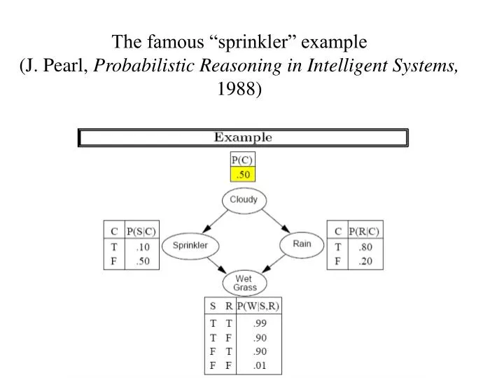
The famous “sprinkler” example(J. Pearl, Probabilistic Reasoning in Intelligent Systems, 1988)
Recall rule for inference in Bayesian networks: Example: What is A (slightly) harder question: What is P(C | W, R)?
Exact Inference in Bayesian Networks General question: What is P(X|e)? Notation convention: upper-case letters refer to random variables; lower-case letters refer to specific values of those variables
General question: Given query variable X and observed evidence variable values e, what is P(X | e)?
Worst-case complexity is exponential in n (number of nodes) • Problem is having to enumerate all possibilities for many variables.
Can reduce computation by computing terms only once and storing for future use. See “variable elimination algorithm” in reading.
In general, however, exact inference in Bayesian networks is too expensive.
... X1 X2X3Xn Approximate inference in Bayesian networks Instead of enumerating all possibilities, sample to estimate probabilities.
Direct Sampling • Suppose we have no evidence, but we want to determine P(C,S,R,W) for all C,S,R,W. • Direct sampling: • Sample each variable in topological order, conditioned on values of parents. • I.e., always sample from P(Xi | parents(Xi))
Example • Sample from P(Cloudy). Suppose returns true. • Sample from P(Sprinkler | Cloudy = true). Suppose returns false. • Sample from P(Rain| Cloudy = true). Suppose returns true. • Sample from P(WetGrass | Sprinkler = false, Rain = true). Suppose returns true. Here is the sampled event: [true, false, true, true]
Suppose there are N total samples, and let NS (x1, ..., xn) be the observed frequency of the specific event x1, ..., xn. • Suppose N samples, n nodes. Complexity O(Nn). • Problem 1: Need lots of samples to get good probability estimates. • Problem 2: Many samples are not realistic; low likelihood.
Markov Chain Monte Carlo Sampling • One of most common methods used in real applications. • Uses idea of Markov blanket of a variable Xi: • parents, children, children’s other parents • Fact: By construction of Bayesian network, a node is conditionally independent of its non-descendants, given its parents.
What is the Markov Blanket of Rain? What is the Markov blanket of Wet Grass? • Proposition: A node Xi is conditionally independent of all other nodes in the network, given its Markov blanket.
Markov Chain Monte Carlo (MCMC) Sampling Algorithm • Start with random sample from variables, with evidence variables fixed: (x1, ..., xn). This is the current “state” of the algorithm. • Next state: Randomly sample value for one non-evidence variable Xi , conditioned on current values in “Markov Blanket” of Xi.
Example • Query: What is P(Rain | Sprinkler = true, WetGrass = true)? • MCMC: • Random sample, with evidence variables fixed: [Cloudy, Sprinkler, Rain, WetGrass] = [true, true, false, true] • Repeat: • Sample Cloudy, given current values of its Markov blanket: Sprinkler = true, Rain = false. Suppose result is false. New state: [false, true, false, true] • Sample Rain, given current values of its Markov blanket: Cloudy = false, Sprinkler = true, WetGrass = true. Suppose result is true. New state: [false, true, true, true].
Each sample contributes to estimate for query P(Rain | Sprinkler = true, WetGrass = true) • Suppose we perform 100 such samples, 20 with Rain = true and 80 with Rain = false. • Then answer to the query is Normalize (20,80) = .20,.80 • Claim: “The sampling process settles into a dynamic equilibrium in which the long-run fraction of time spent in each state is exactly proportional to its posterior probability, given the evidence.” • That is: for all variables Xi, the probability of the value xi of Xi appearing in a sample is equal to P(xi| e). • Proof of claim: Reference on request
Issues in Bayesian Networks • Building / learning network topology • Assigning / learning conditional probability tables • Approximate inference via sampling • Incorporating temporal aspects (e.g., evidence changes from one time step to the next).
Learning network topology • Many different approaches, including: • Heuristic search, with evaluation based on information theory measures • Genetic algorithms • Using “meta” Bayesian networks!
Learning conditional probabilities • In general, random variables are not binary, but real-valued • Conditional probability tables conditional probability distributions • Estimate parameters of these distributions from data • If data is missing on one or more variables, use “expectation maximization” algorithm
Speech Recognition • Task: Identify sequence of words uttered by speaker, given acoustic signal. • Uncertainty introduced by noise, speaker error, variation in pronunciation, homonyms, etc. • Thus speech recognition is viewed as problem of probabilistic inference.
Speech Recognition • So far, we’ve looked at probabilistic reasoning in static environments. • Speech: Time sequence of “static environments”. • Let X be the “state variables” (i.e., set of non-evidence variables) describing the environment (e.g., Words said during time step t) • Let E be the set of evidence variables (e.g., features of acoustic signal).
The E values and X joint probability distribution changes over time. t1: X1, e1 t2: X2 , e2 etc.
At each t, we want to compute P(Words | S). • We know from Bayes rule: • P(S | Words), for all words, is a previously learned “acoustic model”. • E.g. For each word, probability distribution over phones, and for each phone, probability distribution over acoustic signals (which can vary in pitch, speed, volume). • P(Words), for all words, is the “language model”, which specifies prior probability of each utterance. • E.g. “bigram model”: probability of each word following each other word.
Speech recognition typically makes three assumptions: • Process underlying change is itself “stationary” i.e., state transition probabilities don’t change • Current state X depends on only a finite history of previous states (“Markov assumption”). • Markov process of order n: Current state depends only on n previous states. • Values et of evidence variables depend only on current state Xt. (“Sensor model”)
Hidden Markov Models • Markov model: Given stateXt, what is probability of transitioning to next state Xt+1 ? • E.g., word bigram probabilities give P (wordt+1 | wordt ) • Hidden Markov model: There are observable states (e.g., signal S) and “hidden” states (e.g., Words). HMM represents probabilities of hidden states given observable states.
Example: “I’m firsty, um, can I have something to dwink?” From http://www.cs.berkeley.edu/~russell/slides/