Download
1 / 27
270 likes | 381 Views
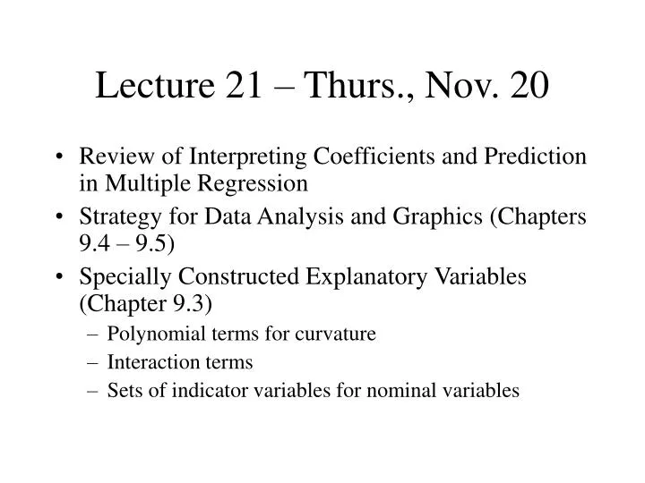
Lecture 21 – Thurs., Nov. 20. Review of Interpreting Coefficients and Prediction in Multiple Regression Strategy for Data Analysis and Graphics (Chapters 9.4 – 9.5) Specially Constructed Explanatory Variables (Chapter 9.3) Polynomial terms for curvature Interaction terms

E N D
Lecture 21 – Thurs., Nov. 20 • Review of Interpreting Coefficients and Prediction in Multiple Regression • Strategy for Data Analysis and Graphics (Chapters 9.4 – 9.5) • Specially Constructed Explanatory Variables (Chapter 9.3) • Polynomial terms for curvature • Interaction terms • Sets of indicator variables for nominal variables
Interpreting Coefficients • Multiple Linear Regression Model • Interpretation of Coefficient : The change in the mean of Y that is associated with increasing Xj by one unit and not changing X1,…,Xj-1, Xj+1,…,Xp • Interpretation holds even if X1,…,Xp are correlated. • Same warning about extrapolation beyond the observed X1,…,Xp points as in simple linear regression.
Coefficients in Mammal Study • It is estimated that • A 1 kg increase in body weight with gestation period and litter size held fixed is associated with a 0.90 g mean increase in brain weight [95% CI: (0.80,1.17)] • A 1 day increase in gestation period with body weight and litter size held fixed is associated with a 1.81g mean increase in brain weight [95% CI : (1.10,2.51)] • A 1 animal increase in litter size with body weight and gestation period held fixed is associated with a 27.65g mean increase in brain weight [95% CI: (-6.94, 62.23)]
Prediction from Multiple Regression • Estimated mean brain weight (=predicted brain weight) for a mammal which has a body weight of 3kg, a gestation period of 180 days and a litter size of 1
Strategy for Data Analysis and Graphics • Strategy for Data Analysis: Display 9.9 in Chapter 9.4 • Good graphical method for initial exploration of data is a matrix of pairwise scatterplots. To display this in JMP, click on Analyze, Multivariate and then put all the variables in Y, Columns.
Specially Constructed Explanatory Variables • The scope of multiple linear regression can be dramatically expanded by using specially constructed explanatory variables: • Powers of the explanatory variables Xjk can be used to model curvature in regression function. • Indicator variables can be used to model the effect of nominal variables • Products of explanatory variables can be used to model interactive effects of explanatory variables
Curved Regression Functions • Linearity assumption in simple linear regression is violated. Transformations wouldn’t work because function isn’t monotonic.
Squared Term for Curvature • Multiple Linear Regression Model:
Terms for Curvature • Two ways to incorporate squared or higher polynomial terms for curvature in JMP • Fit Model, create a variable rainfall2 • Fit Y by X, under red triangle next to Bivariate Fit of Yield by Rainfall, click Fit Polynomial then 2, Quadratic instead of Fit Line (a model with both a squared and cubed term can be fit by clicking 3, Cubic) • Coefficients are not directly interpretable. Change in the mean of Y that is associated with a one unit increase in X depends on X
Interaction Terms • Two variables are said to interact if the effect that one of them has on the mean response depends on the value of the other. • An explanatory variable for interaction can be constructed as the product of the two explanatory variables that are thought to interact.
Interaction in Meadowfoam • Does the effect of light intesnity on mean number of flowers depend on the timing of light regime? • Multiple linear regression model that has term for interaction: • Model is equivalent to • Change in mean of flowers for a one unit increase in light intensity depends on timing onset. • Coefficients are not easily interpretable. Best method for communicating findings with interaction is table or graph of estimated means at various combinations of interacting variables.
Interaction in Meadowfoam • There is not much evidence of an interaction. The p-value for the test that the interaction coefficient is zero is 0.9096.
Displaying Interaction – Coded Scatterplots (Section 9.5.2) • A coded scatterplot is a scatterplot with different symbols to distinguish two or more groups
Coded Scatterplots in JMP • Split the Y variable by the group identity variables (Click Tables, Split, then put Y variable in Split and Group Identity variable in Col ID). • Graph, Overlay Plot, put the columns corresponding to the Y’s for the different group identity variables in Y and put the X variable (light intensity) in X.
Parallel vs. Separate Regression Lines • Model without interaction between time onset and light intensity is a “parallel regression lines” model • Model with interaction is a “separate regression lines” model
Polynomials and Interactions Example • An analyst working for a fast food chain is asked to construct a multiple regression model to identify new locations that are likely to be profitable. The analyst has for a sample of 25 locations the annual gross revenue of the restaurant (y), the mean annual household income and the mean age of children in the area. Data in fastfoodchain.jmp • Relationship between y and each explanatory variable might be quadratic because restaurants attract mostly middle-income households and children in the mid age ranges.
fastfoodchain.jmp results • Strong evidence of a quadratic relationship between revenue and age, revenue and income. Moderate evidence of an interaction between age and income.
Nominal Variables • To incorporate nominal variables in multiple regression analysis, we use indicator variables. • Indicator variable to distinguish between two groups: The time onset (early vs. late is a nominal variable). To incorporate it into multiple regression analysis, we used indicator variable early which equals 1 if early, 0 if late.
Nominal Variables with More than Two Categories • To incorporate nominal variables with more than two categories, we use multiple indicator variables. If there are k categories, we need k-1 indicator variables.
Nominal Explanatory Variables Example: Auction Car Prices • A car dealer wants to predict the auction price of a car. • The dealer believes that odometer reading and the car color are variables that affect a car’s price (data from sample of cars in auctionprice.JMP) • Three color categories are considered: • White • Silver • Other colors • Note: Color is a nominal variable.
Indicator Variables in Auction Car Prices 1 if the color is white 0 if the color is not white I1 = 1 if the color is silver 0 if the color is not silver I2 = The category “Other colors” is defined by: I1 = 0; I2 = 0
Auction Car Price Model • Solution • the proposed model is • The data White car Other color Silver color
Price 16996.48 - .0555(Odometer) 16791.48 - .0555(Odometer) 16701 - .0555(Odometer) Odometer Example: Auction Car Price The Regression Equation From JMP we get the regression equation PRICE = 16701-.0555(Odometer)+90.48(I-1)+295.48(I-2) The equation for a silver color car. Price = 16701 - .0555(Odometer) + 90.48(0) + 295.48(1) The equation for a white color car. Price = 16701 - .0555(Odometer) + 90.48(1) + 295.48(0) Price = 6350 - .0278(Odometer) + 45.2(0) + 148(0) The equation for an “other color” car.
Example: Auction Car Price The Regression Equation From JMP we get the regression equation PRICE = 16701-.0555(Odometer)+90.48(I-1)+295.48(I-2) For one additional mile the auction price decreases by 5.55 cents. A white car sells, on the average, for $90.48 more than a car of the “Other color” category A silver color car sells, on the average, for $295.48 more than a car of the “Other color” category.
There is insufficient evidence to infer that a white color car and a car of “other color” sell for a different auction price. There is sufficient evidence to infer that a silver color car sells for a larger price than a car of the “other color” category. Example: Auction Car Price The Regression Equation Xm18-02b
Shorthand Notation for Nominal Variables • Shorthand Notation for regression model with Nominal Variables. Use all capital letters for nominal variables • Parallel Regression Lines model: • Separate Regression Lines model:
Nominal Variables in JMP • It is not necessary to create indicator variables yourself to represent a nominal variable. • Make sure that the nominal variable’s modeling type is in fact nominal. • Include the nominal variable in the Construct Model Effects box in Fit Model • JMP will create indicator variables. The brackets indicate the category of the nominal variable for which the indicator variable is 1.