Download
1 / 38
430 likes | 842 Views
Chapter 7: Simple Mixtures. Homework: Exercises(a only):7.4, 5,10, 11, 12, 17, 21 Problems: 1, 8. Chapter 7 - Simple Mixtures. Restrictions Binary Mixtures x A + x B = 1, where x A = fraction of A Non-Electrolyte Solutions Solute not present as ions. Partial Molar Quantities -Volume.

E N D
Chapter 7: Simple Mixtures Homework: Exercises(a only):7.4, 5,10, 11, 12, 17, 21 Problems: 1, 8
Chapter 7 - Simple Mixtures • Restrictions • Binary Mixtures • xA + xB = 1, where xA = fraction of A • Non-Electrolyte Solutions • Solute not present as ions
Partial Molar Quantities -Volume • Partial molar volume of a substance slope of the variation of the total volume plotted against the composition of the substance • Vary with composition • due to changing molecular environment • VJ = (V/ nJ) p,T,n’ • pressure, Temperature and amount of other component constant Partial Molar Volumes Water & Ethanol
Partial Molar Quantities & Volume • If the composition of a mixture is changed by addition of dnA and dnB • dV = (V/ nA) p,T,nA dnA + (V/ nB) p,T,nB dnB • dV =VAdnA + VBdnB • At a given compositon and temperature, the total volume, V, is • V = nAVA + nBVB
Measuring Partial Molar Volumes • Measure dependence of volume on composition • Fit observed volume/composition curve • Differentiate Example - Problem 7.2 For NaCl the volume of solution from 1 kg of water is: V= 1003 + 16.62b + 1.77b1.5 + 0.12b2 What are the partial molar volumes? VNaCl = (∂V/∂nNaCl) = (∂V/∂nb) = 16.62 + (1.77 x 1.5)b0.5 + (0.12 x 2) b1 At b =0.1, nNaCl = 0.1 VNaCl = 16.62 + 2.655b0.5 + 0.24b = 17.48 cm3 /mol V = 1004.7 cm3 nwater = 1000g/(18 g/mol) = 55.6 mol V = nNaClVNaCl + nwaterVwater Vwater = (V - VNaCl nNaClr )/ nwater = (1004.7 -1.75)/55.6= 18.04 cm3 /mol
Partial Molar Quantities - General • Any extensive state function can have a partial molar quantity • Extensive property depends on the amount of a substance • State function depends only on the initial and final states not on history • Partial molar quantity of any function is just the slope (derivative) of the function with respect to the amount of substance at a particular composition • For Gibbs energy this slope is called the chemical potential, µ
Partial Molar Free Energies • Chemical potential, µJ, is defined as the partial molar Gibbs energy @ constant P, T and other components • µJ = (G/ nJ) p,T,n’ • For a system of two components: G = nAµA + n B µB • G is a function of p,T and composition • For an open system constant composition, dG =Vdp - SdT + µA dnA + µB dn B • Fundamental Equation of Thermodynamics • @ constant P and T this becomes, dG = µA dnA + µB dn B • dG is the the non expansion work, dwmax • FET implies changing composition can result in work, e.g. an electrochemical cell
Chemical Potential • Gibbs energy, G, is related to the internal energy, U U = G - pV + TS (G = U + pV - TS) • For an infinitesimal change in energy, dU dU = -pdV - Vdp + TdS + SdT + dG but dG =Vdp - SdT + µA dnA + µB dn B so dU = -pdV - Vdp +TdS +SdT + Vdp - SdT + µA dnA + µB dn B dU = -pdV + TdS + µA dnA + µB dn B at constant V and S, dU = µA dnA + µB dn B or µJ = (U/ nJ)S,V,n’
µ and Other Thermodynamic Properties • Enthalpy, H (G = H - TS) dH = dG + TdS + SdT dH= (Vdp - SdT + µA dnA + µB dn B) - TdS SdT dH = VdP - TdS + µA dnA + µB dn B at const. p & T : dH = µA dnA + µB dn B or µJ = (H/ nJ)p,T,n’ • Helmholz Energy, A (A = U-TS) dA = dU - TdS - SdT dA = (-pdV + TdS + µA dnA + µB dn B ) - TdS - SdT dA = -pdV - SdT + µA dnA + µB dn B at const. V & T : dA = µA dnA + µB dn B or µJ = (A/ nJ)V,T,n’
Gibbs-Duhem Equation • Recall, for a system of two components: G = nAµA + n B µB • If compositions change infinitesimally dG = µA dnA + µB dn B + nAdµA + n Bd µB • But at constant p & T, dG = µA dnA + µB dn B so µA dnA + µB dn B = µA dnA + µB dn B + nAdµA + n Bd µB or nAdµA + n Bd µB = 0 • For J components, nidµi = 0 (i=1,J) {Gibbs-Duhem Equation}
Significance of Gibbs-Duhem • Chemical potentials of multi-component systems cannot change independently • Two components, G-D says, nAdµA + n Bd µB = 0 • means that d µB = (nA/ n B)dµA • Applies to all partial molar quantities • Partial molar volume dVB = (nA/ n B)dVA • Can use this to determine on partial molar volume from another • You do this in Experiment 2
Example Self Test 7.2 VA = 6.218 + 5.146b - 7.147b2 dVA = + 5.146 - 2*7.147b = + 5.146 - 14.294b db dVA/db = + 5.146b - 14.294b If *MB is in kg/mol dVB = -nA/nB (dVA); b=nA/nB*MB or b *MB = nA/nB dVB = -nA/nB (dVA ) = nA/nB dVA = b *MB dVA dVB = -b* MB (5.146 - 14.294b) db =- MB(2.573b-4.765b2) VB =VB* + MB (4.765b2 - 2.573b) from data VB* = 18.079 cm3mol-1 and MB = 0.018 kg/mol so VB = 18.079 cm3mol-1 + 0.0858b2 - 0.0463b
Gibbs Energy of Mixing Of Two Ideal Gases Thermodynamics of Mixing • For 2 Gases (A &B) in two containers, the Gibbs energy, Gi Gi = nAµA + nBµB • But µ = µ° + RTln(p/p°) so Gi = nA(µA° + RTln(p/p°) )+ nB(µB° + RTln(p/p°)) • If p is redefined as the pressure relative to p° Gi = nA(µA° + RTln(p) )+ nB(µB° + RTln(p) ) • After mixing, p = pA + pB and Gf = nA(µA° + RTln(pA) )+ nB(µB° + RTln(pB) ) • So Gmix = Gf - Gi = nA (RTln(pA/p) )+ nB(RTln(pB /p) • Replacing nJ by xJn and pJ/p=xJ (from Dalton’s Law) Gmix = nRT(xA ln (xA ) + xBln(xB )) • This equation tells you change in Gibbs energy is negative since mole fractions are always <1
Example :Self-Test 7.3 • 2.0 mol H2(@2.0 atm) + 4 mol N2 (@3.0 atm) mixed at const. V. What is Gmix? Initial: pH2= 2 atm;VH2= 24.5 L; pN2= 3 atm;VN2= 32.8 L{Ideal Gas} Final: VN2= VH2= 57.3 L; therefore pN2= 1.717 atm; pH2= 0.855 atm;{Ideal Gas} Gmix = RT(nA ln (pA /p) + nBln(pB /p)) Gmix = (8.315 J/mol K)x(298 K)[2mol x ( ln(0.855/2) + 4 mol x (ln(1.717/3)] Gmix = -9.7 J What is Gmix under conditions of identical initial pressures? xH2 = 0.333; xN2 = 0.667; n = 6 mol Gmix = nRT(xA ln (xA ) + xBln(xB )) Gmix = 6mol x( 8.315J/molK)x 298.15K{0.333ln0.333 +0.667ln0.667) Gmix = -9.5 J
Entropy of Mixing Two Ideal Gases Entropy and Enthalpy of Mixing • For Smix, recall G = H - TS Therefore Smix = -Gmix / T Smix = - [ nRT(xA ln (xA ) + xBln(xB ))] / T Smix = - nR(xA ln (xA ) + xBln(xB ) • It follows that Smix is always (+) since xJln(xJ ) is always (-) • For Hmix H = G + TS ={nRT(xA ln (xA ) + xBln(xB )} +T{- nR(xA ln (xA ) + xBln(xB )} H ={nRT(xA ln (xA ) + xBln(xB )} - {nRT(xA ln (xA ) + xBln(xB )} H = 0 • Thus driving force for mixing comes from entropy change
Chemical Potentials of LiquidsIdeal Solutions • At equilibrium chem. pot. of liquid = chem. pot. of vapor, µA(l) = µA(g,p) • For pure liquid, µ*A(l) = µ°A + RT ln(p *A) [1] • For A in solution, µA(l) = µ°A + RT ln(p A) [2] • Subtracing [1] from [2] : µA(l) - µ*A(l) = RT ln(pA) + RT ln(p *A) µA(l) - µ*A(l) = RT{ln(pA) - ln(p *A)} = RT{ln(pA/p *A)} µA(l) = µ*A(l) + RT{ln(pA/p *A)} [3] • Raoult’s Law - ratio of the partial pressure of a component of a mixture to its vapor pressure as a pure substance (pA/p*A) approximately equals the mole fraction, xA pA = xA p*A • Combining Raoult’s law with [3] gives µA(l) = µ*A(l) + RT{ln(xA)}
Ideal Solutions/Raoult’s Law • Mixtures which obey Raoult’s Law throughout the composition range are Ideal Solutions • Phenomenology of Raoult’s Law: 2nd component inhibits the rate of molecules leaving a solution, but not returning • rate of vaporization XA • rate of condensation pA • at equilibrium rates equal • implies pA = XA p*A
Deviations from Raoult’s Law • Raoult’s Law works well when components of a mixture are structurally similar • Wide deviations possible for dissimilar mixtures • Ideal-Dilute Solutions • Henry’s Law (William Henry) • For dilute solutions, v.p. of solute is proportional to the mole fraction (Raoult’s Law) but v.p. of the pure substance is not the constant of proportionality • Empirical constant, K, has dimensions of pressure • pB = xBKB (Raoult’s Law says pB = xBpB) • Mixtures in which the solute obeys Henry’s Law and solvent obeys Raoult’s Law are called Ideal Dilute Solutions • Differences arise because, in dilute soln, solute is in a very different molecular environment than when it is pure
Applying Henry’s Law & Raoult’s Law • Henry’s law applies to the solute in ideal dilute solutions • Raoult’s law applies to solvent in ideal dilute solutions and solute & solvent in ideal solutions • Real systems can (and do ) deviate from both
Applying Henry’s Law • What is the mole fraction of dissolved hydrogen dissolved in water if the over-pressure is 100 atmospheres? Henry’s constant for hydrogen is 5.34 x 10⁷ PH2= xH2K; xH2 = PH2 /K= 100 atm x 760 Torr/atm/ 5.34 x 10⁷ xH2 = 1.42 x 10⁻³ In fact hydrogen is very soluble in water compared to other gases, while there is little difference between solubility in non-polar solvents. If the solubility depends on the attraction between solute and solvent, what does this say about H2 -water interactions?
Properties of Solutions • For Ideal Liquid Mixtures • As for gases the ideal Gibbs energy of mixing is Gmix = nRT(xA ln (xA ) + xBRTln(xB )) • Similarly, the entropy of mixing is Smix = - nR(xA ln (xA ) + xBln(xB ) and Hmix is zero • Ideality in a liquid (unlike gas) means that interactions are the same between molecules regardless of whether they are solvent or solute • In ideal gases, the interactions are zero
Real Solutions • In real solutions, interactions between different molecules are different • May be an enthalpy change • May be an additional contribution to entropy (+ or - ) due to arrangement of molecules • Therefore Gibbs energy of mixing could be + • Liquids would separate spontaneously (immiscible) • Could be temperature dependent (partially miscible) • Thermodynamic properties of real solns expressed in terms of ideal solutions usingexcess functions • Entropy: SE = Smix - Smixideal • Enthalpy: HE = Smix(because Hmixideal = 0) • Assume HE = nbRTxAxB where is const. b =w/RT • w is related to the energy of AB interactions relative to AA and BB interactions • b > 0, mixing endothermic; b < 0, mixing exothermic solvent-solute interactions more favorable than solvent-solvent or solute-solute interactions • Regular solution is one in which HE 0 but SE 0 • Random distribution of molecules but different energies of interactions • GE = HE • Gmix = nRT{(xA ln (xA ) + xBRTln(xB )) + bRTxAxB (Ideal Portion + Excess)
Activities of Regular Solutions • Recall the activity of a compound, a, is defined a = gx where g = activity coefficient • For binary mixture, A and B, consideration of excess Gibbs energy leads to the following relationships (Margules’ eqns) ln gA = bxB2 and ln gB = bxA2 [1] • As xB approaches 0, gA approaches 1 • Since, aA = gAxA, from [1] • If b = 0, this is Raoult’s Law • If b < 0 (endothermic mixing), gives vapor pressures lower than ideal • If b > 0 (exothermic mixing), gives vapor pressures higher than ideal • If xA<<1, becomes pA = xAeb pA* • Henry’s law with K = eb pA*
Colligative Properties • Properties of solutions which depend upon the number rater than the kind of solute particles • Arise from entropy considerations • Pure liquid entropy is higher in the gas than for the liquid • Presence of solute increases entropy in the liquid (disorder increases) • Lowers the difference in entropy between gas and liquid hence the vapor pressure of the liquid • Result is a lowering chemical potential of the solvent • Types of colligative properties • Boiling Point Elevation • Freezing Point Depression • Osmotic pressure
Colligative Properties - General • Assume • Solute not volatile • Pure solute separates when frozen • When you add solute the chemical potential, µA becomes µA = µA * + RT ln(xA) where µA * = Chemical Potential of Pure Substance x A = mole fraction of the solvent • Since ln(xA) in negative µA > µA*
Boiling Point Elevation At equilibrium µ(gas) = µ(liquid) or µA(g) = µA *(l) + RTln(xA) Rearranging,(µA(g) - µA *(l))/RT = ln(xA) = ln(1- xB) But , (µA(g) - µA *(l)) = G vaporization so ln(1- xB) = G vap. /RT Substituting for G vap. (H vap. -T S vap. ) {Ingnore T dependence of H & S) ln(1- xB) = (H vap. -T S vap.)/RT = (H vap. /RT) - S vap./R When xB = 0 (pure liquid A), ln(1) = (H vap. /RTb) - S vap./R = 0 or H vap. /RTb = S vap./R where Tb= boiling point Thus ln(1- xB) = (H vap. /RT) - H vap. /RTb = (H vap. /R)(1/T- 1/Tb) If 1>> xB, (H vap. /R)(1/T- 1/Tb) - xB and if T Tb and T= T Tb Then (1/T- 1/Tb) = T/Tb2 and (H vap./R) T/Tb2 = - xB so T= - xB Tb2 /(H vap./R) or T= - xB Kb where Kb = Tb2 /(H vap./R)
Boiling Point Elevation • Kb is the ebullioscopic constant • Depends on solvent not solute • Largest values are for solvents with high boiling points • Water (Tb = 100°C) Kb = 0.51 K/mol kg -1 • Acetic Acid (Tb = 118.1°C) Kb = 2.93 K/mol kg -1 • Benzene (Tb = 80.2°C) Kb = 2.53 K/mol kg-1 • Phenol (Tb = 182°C) Kb = 3.04 K/mol kg -1
Freezing Point Depression • Derivation the same as for boiling point elevation except • At equilibrium µ(solid) = µ(solid) or µA(g) = µA *(l) + RTln(xA) • Instead of the heat of vaporization, we have heat of fusion • Thus, T= - xB Kf where Kf = Tf2 /(H fus./R) • Kf is the cryoscopic constant • Water (Tf = 0°C) Kf = 1.86 K/mol kg -1 • Acetic Acid (Tf = 17°C) Kf = 3.9 K/mol kg -1 • Benzene (Tf = 5.4°C) Kf = 5.12 K/mol kg-1 • Phenol (Tf = 43°C) Kf = 7.27 K/mol kg -1 • Again property depends on solvent not solute
Temperature Dependence of Solubility • Not strictly speaking colligative property but can be estimated assuming it is • Starting point the same - assume @ equilibrium µ is equal for two states • First state is solid solute, µB(s) • Second state is dissolved solute, µB(l) • µB(l) = µB*(l) + RT ln xB • At equilibrium, µB(s) = µB(l) • µB(s) = µB*(l) + RT ln xB • Same as expression for freezing point except that use xB instead of xA
Temperature Dependence of Solubility • To calculate functional form of temperature dependence you solve for mole fraction • ln xB = [µB(s) - µB*(l)]/ RT = -G fusion/RT = -[H fus-T S fus]/RT • ln xB = -[H fus-T S fus]/RT = -[H fus /RT] + [S fus/R] {1} • At the melting point of the solute, Tm, G fusion/RTm = 0 because G fusion = 0 • So [H fus-TmS fus]/RTm = 0 or [H fus /RTm] -[S fus/R] = 0 • Substituting into {1}, ln xB = -[H fus /RT] + [S fus/R]+ [H fus /RTm] -[S fus/R] • This becomes ln xB = -[H fus /RT] + [H fus /RTm] • Or ln xB = -[H fus /R] [1/T - 1/Tm] • Factoring Tm, ln xB = [H fus /R Tm] [1 - (Tm /T)] • Or xB = exp[H fus /R Tm] [1 - (Tm /T)-1] • The details of the equation are not as important as functional form • Solubility is lowered as temperature is lowered from melting point • Solutes with high melting points and large enthalpies of fusion have low solubility • Note does not account for differences in solvent - serious omission
ln xB = -[H fus /R] [1/T - 1/Tm] or xB = exp[H fus /R Tm] [1 - (Tm /T)-1]
Osmotic pressure • J. A. Nollet (1748) - “wine spirits” in tube with animal bladder immersed in pure water • Semi-permiable membrane - water passes through into the tube • Tube swells , sometimes bladder bursts • Increased pressure called osmotic pressure from Greek word meaning impulse • W. Pfeffer (1887) -quantitative study of osmotic pressure • Membranes consisted of colloidal cupric ferrocyanide • Later work performed by applying external pressure to balance the osmotic pressure • Osmotic pressure , , is the pressure which must be applied to solution to stop the influx of solvent
Osmotic Pressure van’t Hoff Equation • J. H. van’t Hoff (1885) - In dilute solutions the osmotic pressure obeys the relationship, V=nBRT • nB/V = [B] {molar concentration of B, so =[B] RT • Derivation- at equilibrium µ solvent is the same on both sides of membrane: µA *(p) = µA (x A,p +) {1} • µA (x A,p +) = µ*A (x A,p +) + RTln(x A) {2} • µ*A (x A,p +) = µA *(p) + ∫pp +Vm dp {3} [Vm = molar volume of the pure solvent] • Combining {1} and {2} : µA *(p) = µA *(p) + ∫pp +Vm dp + RTln(x A) • For dilute solutions, ln(x A) = ln(x B) ≈ - x B • Also if the pressure range of integration is small, ∫pp +V m dp = Vm∫pp +dp = Vm • So 0 = V m + RT - x B or Vm= RT x B • Now nA V m = V and, if solution dilute x B ≈ - n B /nA so =[B] RT • Non-ideality use a virial expansion • =[B] RT{1 + B[B] + ...} where B I s the osmotic virial coef. (like pressure)
Application of Osmotic Pressure • Determine molar mass of macromolecules • =[B] RT{1 + B[B] + ...} but [B] = c/M where c is the concentration and M the molar mass so • = c/M RT{1 + Bc/M + ...} • g h = c/M RT{1 + Bc/M + ...} • h/c = RT/(Mg) {1 + Bc/M + ...} • h/c = RT/(Mg) + RTB/(M2g) + ...} • Plot of h/c vs. c has intercept of RT/(Mg) so • Intercept= RT/(Mg) or M= RT/(intercept xg) • Units (SI) are kg/mol typical Dalton (Da) {1Da = 1g/ mol
Non-Ideality & ActivitiesSolvents • Recall for ideal solution µA =µA * + RTln(xA) • µA* is pure liquid at 1 bar when xA =1 • If solution does not ideal xA can be replaced with activity aA • activtiy is an effective mole fraction • aA = pA/pA* {ratio of vapor pressures} • Because for all solns µA =µA * + RTln(pA/ p*A) • As xA-> 1, aA -> xA so define activity coefficient,, such that • aA = A xA • As xA-> 1, A -> 1 • Thus µA =µA * + RTln(xA) + RTln(A) {substiuting for a A}
Non-Ideality & ActivitiesSolutes (Ideal & Non-Ideal) • For ideal dilute solutions Henry’s Law ( pB = KBxB) applies • Chemical potential µB = µB * + RTln(pB /pB*) • µB = µB * + RTln(KBxB /pB*) = µB * + RTln(KB/pB*) + RTln(xB ) • KB and pB* are characteristics of the solute so you can combine them with µB * µB† = µB * + RTln(KBxB /pB*) • Thus µB = µB† + RTln(xB ) • Non-ideal solutes • As with solvents introduce acitvity and activity coefficient • aB = pB/KB*; aB = B xB • As xA-> 0, aA -> xA and A -> 1
Activities in Molalities • For dilute solutions x B ≈ n B /nA , and x B = b/b° • kappa, , is a dimensionless constant • For ideal-dilute solution, µB = µB† + RTln(xB ) so µB = µB† + RTln( b/b°) = µB†+ RTln() + RTln( b/b°) • Dropping b° and combing 1st 2 terms, µB = µBø+ RTln( b) • µBø = µB†+ RTln() • µB has the standard value (µBø ) when b=b° • As b ->0, µB ->infinity so dilution stabilizes system • Difficult to remove last traces of solute from a soln • Deviations from ideality can be accounted for by defining an activity aB and activity,B, • aB = B bB/b° where B ->1, bB -> 0 • The chemical potential then becomes µ = µø + RTln( a) • Table 7.3 in book summarizes the relationships