Download
1 / 57
580 likes | 707 Views
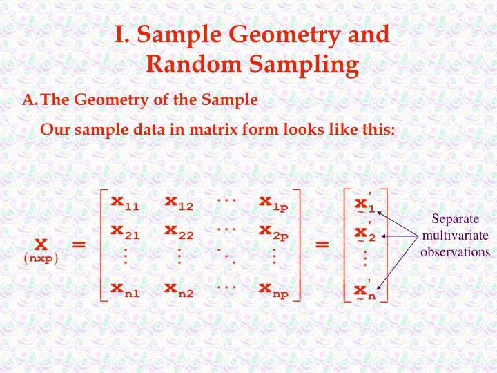
I. Sample Geometry and Random Sampling. A. The Geometry of the Sample Our sample data in matrix form looks like this:. Separate multivariate observations.

E N D
I. Sample Geometry and Random Sampling A. The Geometry of the Sample Our sample data in matrix form looks like this: Separate multivariate observations
Just as the point where the population means of all p variables lies is the centroid of the population, the point where the sample means of all p variables lies is the centroid of the sample – for a sample with two variables and three observations: we have x2 row space centroid of the sample x11,x12 _ _ x•1,x•2 x31,x32 x21,x22 x1 in the p = 2 variable or ‘row’ space (because rows are treated as vector coordinates)
These same data plotted in item or ‘column’ space, would like like this: 3 column space centroid of the sample x11,x21 ,x31 _ _ _ 2 x1•,x2•,x3• x12,x22 ,x32 This is referred to as the ‘column’ space because columns are treated as vector coordinates)
Suppose we have the following data: In row space we have the following p = 2 dimensional scatter diagram x2 x21,x22 row space centroid of the sample (1,7) x11,x12 x1 with the obvious centroid (1,7).
For the same data: In column space we have the following n = 2 dimensional plot 2 x12,x22 row space centroid of the sample (4,4) 1 x11,x21 with the obvious centroid (4,4).
Suppose we have the following data: in row space we have the following p = 3 dimensional scatter diagram x3 x31,x32,x33 row space centroid of the sample x11,x12,x13 (-1,4,5) x1 x21,x22,x23 x2 with the centroid (-1,4,5).
For the same data: in column space we have the following n = 3 dimensional scatter diagram 3 x13,x23,x33 (4,3,1) 1 x12,x22,x32 2 with the centroid (4,3,1). x11,x21,x31
The column space reveals an interesting geometric interpretation of the centroid – suppose we plot an n x 1 vector 1: ~ 3 In n = 3 dimensions we have: 1,1,1 1 2 This vector obviously forms equal angles with each of the n coordinate axes – this means normalization of this vector yields
Now consider some vector yi of coordinates (that represent various sample values of a random variable X). ~ 3 x1,x2,x3 In n = 3 dimensions we have: 1 2
The projection of yi on the unit vector is given by ~ 3 In n = 3 dimensions we have: yi ~ 1 1 ~ 2 _ The sample mean xi corresponds to the multiple of 1 necessary to generate the projection of yi onto the line determined by 1! ~ ~ ~
Again using the Pythagorean Theorem, we can show that the length of the vector drawn perpendicularly from the projection of y onto 1 to y is . ~ 3 In n = 3 dimensions we have: yi ~ 1 1 ~ 2 This is often referred to as the deviation (or mean corrected) vector and is given by:
Example: Consider our previous matrix of three observations in three-space: This data has a mean vector of: _ _ _ i.e., x1 = -1.0, x2 = 4.0, and x3 = 5.0.
Consequently _ Note here that xi1 dii =1 ,…,p . ~ ~
We are particularly interested in the deviation vectors If we plot these deviation (or residual) vectors (translated to the origin without change in their lengths or directions) 3 1 2
Now consider the squared lengths of the deviation vectors: squared length of deviation vector sum of the squared deviations Recalling that the sample variance is: we can see that the squared length of a variable’s deviation vector is proportional to that variable’s variance (and so length is proportional to the standard deviation)!
Now consider any two deviation vectors. Their dot product is which is simply a sum of crossproducts. Now let qik denote the angle between these two deviation vectors. Recall that by substitution we have that
Another substitution based on and yields
Example: Consider our previous matrix of three observations in three-space: which resulted in deviation vectors Let’s use these results to find the sample covariance and correlation matrices.
so: which gives us
B. Random Samples and the Expected Values of m and S Suppose we intend to collect n sets of measurements (or observations) on p variables. At this point we can consider each of the n x p values to be observed to be random variables Xjk. This leads to interpretation of each set of measurements Xj on the p variables to be a random vector, i.e., ~ ~ ~ Separate multivariate observations These concepts will be used to define a random sample.
Random Sample – if the row vectors - represent independent observation - from a common joint probability distribution then are said to form a random sample from . This means the observations have a joint density function of
Keep in mind two thoughts with regards to random samples - The measurements of the p variables in a single trial will usually be correlated. The measurements from different trials, however, must be independent for inference to be valid. - Independence of the measurements from different trials is often violated when the data have a serial component.
Note that m and S have certain properties no matter what the underlying joint distribution of random variables is. Let ~ ~ be a random sample from a joint distribution with mean vector m and covariance matrix S. Then: - X is an unbiased estimate of m, i.e., E(X) = m, and has a covariance matrix - the sample covariance matrix Sn has expected value ~ ~ _ ~ ~ ~ ~ ~ bias i.e., Sn is a biased estimator of covariance matrix S, but ~ ~
This means we can write an unbiased sample variance covariance matrix S as ~ whose (i,k)th element is
Example: Consider our previous matrix of three observations in three-space: the unbiased estimate S is ~
Notice that this does not change the sample correlation matrix R! Why?
C. Generalizing Variance over P Dimensions For a given variance-covariance matrix the Generalized Sample Variance is |S|. ~
Example: Consider our previous matrix of three observations in three-space: the Generalized Sample Variance is
Of course, some of the information regarding the variances and covariances is lost when summarizing multiple dimensions with a single number. Consider the geometry of |S| in two dimensions - we will generate two deviation variables ~ Q This resulting trapezoid has area .
Because sin2(q) + cos2(q) = 1, we can rewrite the area of this trapezoid as Earlier we showed that and cos(q) = r12.
So by substitution and we know that So .
More generally, we can establish the Generalized Sample Variance to be which simply means that the generalized sample variance (for a fixed set of data) is proportional to the squared volume generated by its p deviation vectors. Note that - the generalized sample variance increases as any deviation vector increases in length (the corresponding variable increases in variation) - the generalized sample variance increases as the direction of any two deviation vector becomes more dissimilar (the correlation of the corresponding variables decreases)
Here we see the generalized sample variance changes as the length of deviation vector d2 changes (the variation of the corresponding variable changes): 3 3 1 1 2 2 deviation vector d2 increases in length to cd2 , c > 1 (i.e., the variance of x2 increases)
Here we see the generalized sample variance decrease as the direction of deviation vectors d2 and d3 become more similar (the correlation of x2 and x3 increases): 3 3 1 1 2 2 q23 = 900, i.e., deviation vectors d2 and d3 are orthogonal (x2 and x3 are not correlated 00< q23 < 900, i.e., deviation vectors d2 and d3 move in similar directions (x2 and x3 are positively correlated
This suggests an important result - the generalized sample variance is zero when and only when at least one deviation vector lies in the span of other deviation vectors, i.e., when. one deviation vector is a linear combination of some other deviation vectors one variable is perfectly correlated with a linear combination of other variables the rank of the data is less than the number of columns the determinant of the variance-covariance matrix is zero
These results also suggests simple conditions for determining if S is of full rank: - If n p then |S| = 0 - For the p x 1 vectors x1, x2, …, xp representing realizations of independent random vectors X1, X2, …, Xp, where xj’ is the jth row of data matrix X ~ ~ ~ ~ ~ ~ ~ ~ ~ ~ if the linear combination a’Xj has positive variance for each constant vector a 0 and p < n, S is of full rank and |S| > 0 if a’Xj is a constant j, then |S| = 0 ~ ~ ~ ~ ~ ~ ~ ~ ~
Generalized Sample Variance also has a geometric interpretation in the p-dimensional scatter plot representation of the data in row space. Consider the measure of distance of each point in row space from the sample centroid with S-1 substituted for A. Under these circumstances, the coordinates x’ that lie a constant distance c from the centroid must satisfy ~ ~ ~
A little integral calculus can be used to show that the volume of this ellipsoid is where Thus, the squared volume of the ellipsoid is equal to the product of some constant and the generalized sample variance.
Example: Here we have three data sets, all with centroid (3, 3) and generalized variance |S| = 9.0: ~ Data Set A
Other measures of Generalized Variance have been suggested based on: - the variance-covariance matrix of the standardized variables, i.e., |R| - total sample variance, i.e., ignores differences in variances of individual variables ~ ignores pairwise correlations between variables
D. Matrix Operations for Calculating Sample Means, Covariances, and Correlations For a given data matrix X ~ we have that
We can also create a n x p matrix of means If we subtract this result from data matrix X we have ~ which is an n x p matrix of deviations!
Now the matrix (n – 1)S of sums of squares and crossproducts is ~