Download
1 / 34
340 likes | 478 Views
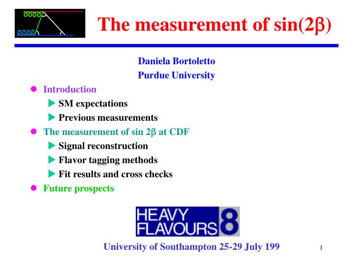
The measurement of sin(2 ). Daniela Bortoletto Purdue University Introduction SM expectations Previous measurements The measurement of sin 2 at CDF Signal reconstruction Flavor tagging methods Fit results and cross checks Future prospects. University of Southampton 25-29 July 199.

E N D
The measurement of sin(2) Daniela Bortoletto Purdue University • Introduction • SM expectations • Previous measurements • The measurement of sin 2 at CDF • Signal reconstruction • Flavor tagging methods • Fit results and cross checks • Future prospects University of Southampton 25-29 July 199
Introduction • SM with 3 generations and the CKM ansatz can accomodate CP if the complex phase is 0CP. Only =0.21960.023, A=0.8190.035 are measured precisely. • CP is one of the less well-tested parts of SM ( , / in the Kaon system) • CP asymmetries in the B system are expected to be large. Independent observations of CP in the B system can: • test the SM • lead to the discovery of new physics
B0-B0 mixing B/ (,) (+i) (1--i) BK (0,0) (1,0) B Physics and CKM matrix Vud Vub*+Vcd Vcb*+Vtd+Vtb*=0 • The goal of B-physics is to over-constrain the unitarity triangle to test the CKM ansatz or to expose new physics B BJ/K0s Unitarity triangle
V*td f f B0 B0 t b d W B0 W B0 t b d B0 B0 CP violation in B decays Box Diagram • Possible manifestations of CP violation can be classified as: • CP violation in the decay: It occurs in B0/B+decays if |A(f)/|A(f)|1 • CP violation in mixing: It occurs when the neutral mass eigenstates are not CP eigenstates (|q/p|1) • CP violation in the interference between decays with and without mixing • Mixing: Vtd introduces a complex phase in the box diagram • Interfering amplitudes: • direct decay B0f • B0 B0 mixing followed by B0 f Vtd
Determination of sin(2) • Color suppressed modes bccs. Dominant penguin contribution has the same weak phase Negligible theoretical uncertainty • Cabibbo suppressed modes bccd such as B0/B0 DD,D*D*. Large theoretical uncertainties due to the penguin contribution • Penguin only or penguin dominated modes bsss or dds. Tree contributions absent or Cabbibbo and color suppressed penguin diagrams dominate even larger theoretical uncertainties
ACP(t) t Experimental considerations • B-factories at the (4S): • B0 and B0 mesons are produced in a coherent C=-1 state time integrated CP asymmetry = 0. • Determination of CP needs A(t ) where t=t(CP)-t(tag) or z =c t • Need good z resolution • pp and pp colliders: time integrated asymmetry does not vanish Since xd=0.732 0.0032 (PDG98) ACP is Maximum at t=2.2 lifetimes • Measurement of the asymmetry as a function of proper time ACP(t) is more powerful • Combinatoric background dominates small ct region
B0/B0J/K0s • For B0/B0 J/K0S we have CP(K0s)=1 and CP(J/K0S )= -1. To reach a common final state the K0 must mix additional phase • Asymmetry is directly related to sin2. ACP(t)=sin[2(M- D)]sin mdt =sin2 sin mdt and sin2 = K0-K0 mixing B0 B0 Mixing Ratio of
Indirect determination of sin2 • Vub/Vcb=0.093from semileptonic decays • K=2.2810-3 • B0-B0 mixing md=0.472 ps-1 • Limit on Bs-Bs mixing ms >12.4 ps-1 • In SM the asymmetries in the B system are expected to be large • S. Mele CERN-EP-98-133, 1998 finds sin2=0.75 0.09 • Parodi et al. sin2=0.725 0.06 • Ali et al. 0.52<sin2<0.94
Measurement accuracy • Measurement of ACP(t) requires: • Reconstruct the signal B0/B0J/K0S • Measure proper decay time (not critical in pp colliders but useful) • Flavor tagging to determine if we have a B0(bd) or B0(bd) at production • Tagging algorithms are characterized by an efficiency and a dilution D. The measured asymmetry isAobsCP=D ACP • Ntot = total number of events • NW= number of wrong tags • NR=number of right tags • D=2P-1 (P=prob. of correct tag) and D=1 if NW=0 D=0 if NW=NR • Best tagging methods has highest D2 Crucial factor
Tagging • Assume you have 200 events N=200 • 100 are tagged Ntag=100 • tagging efficiency =Ntag/Ntot=50% • Of those 100 events • 60 are right sign NR=60 • 40 are wrong signNW=40 • Dilution • D=(NR-NW)/(NR+NW)=(60-40)/100=20% • Effective tagging efficiency • D2=(0.5)(0.2)2=2% • Statistical power of this sample • ND2=200*0.02=4 events
Previous Measurements • Opal Zbb D. Ackerstaff et al. Euro. Phys. Jour. C5, 379 (1998) (Jan-1998) 24 J/K0S candidates Purity 60 % • Flavor tagging techniques: • Jet charge on opposite side jet • Jet charge on same side B • Vertex charge of a significantly separated vertex in the opposite hemisphere sin2=3.2 0.5 1.8 2.0
Previous Measurements • CDF ppbb Abe et al. PRL. 81, 5513 (1998) (June 1998) • 198 17 B0/B0 J/K0S candidates with both muons in the SVX ( S/B 1.2). Measure asymmetry withSame side tagging • Dsin2=0.31 1.1 0.3. • Using D=0.166 0.018 (data) 0.013 (MC) from mixing measurement + MC sin2=1.8 1.1 0.3
Run I CDF detector • Crucial components for B physics: • Silicon vertex detector proper time measurements • impact parameter resolution: d=(13+40/pT) m • typical 2D vertex error (r-)60 m • Central tracking chamber mass resolution. B=1.4T, R=1.4m (pT/pT)2=(0.0066)2(0.0009pT)2 typical J/K0Smass resolution 10 MeV/c2 • Lepton detection (triggering and tagging)
CDF updated measurement • Add candidate events not fully reconstructed in the SVX • Double the signal to 400 events but additional signal has larger (ct) • Use more flavor tag methods to establish b flavor at production • Check D2 with mixing analysis • Use a maximum likelihood method to combine the tags. Weight the events: • in mass (B peak versus sidebands) • in lifetime (more analyzing power at longer lifetimes) • in tagging probability • Account for detector biases background B c (B0)=1.5610-12 s
+ - + - B decay primary J/K0SEvent selection • Signal • J/ -+require two central tracks with matching hits in the muon chambers • K0S -+use long lifetime c(K0S)=2.7 cm to reject background by requiring Lxy/(Lxy)>5 • Perform 4-track fit assuming B J/ K0S • Constrain -+and -+to m(K0S) and m(J/) world average respectively • K0S points to B vertex and B points to primary vertex • Background • cc production prompt J/ ( not from b decays) + random K0S or fake • bb production J/+X, random K0S or fake
J/K0SSignal sample Both in SVX • CDF run1, L=110 pb-1 • 202 events with both muons in SVX(ct) 60 m. • 193 with one or both muons NOT in SVX (ct) 300-900 m 202 18 events 395 31 events S/B=0.9 One or Both not in SVX 19326 S/B=0.7 S/B=0.5 • Plot normalized mass M-MB/ error on M
Flavor tagging methods • We must determine if we had a B0 or a B0 at the time of production. • Opposite-side flavor tagging (OST) bb produced by QCD Identify the flavor of the other b in the event to infer the flavor of the B0 /B0 J/K0S. At CDF 60% loss in efficiency due the acceptance of the other B0. • Lepton tagging : • b +X b • b -X b • Jet charge tag : • Q(b-jet) > 0.2 b • Q(b-jet) <- 0.2 b B0(bd) J/K0S + - + K0S - Opposite side b + Q(b-jet)>0.2
Jet Charge Flavor tagging Qjet in BJ/K • Identify the flavor of the B0/B0J/K0Sthrough the charge of the opposite b-jet • Jet definition allows for wide low PT jets: • Cluster tracks by invariant mass (Invariant mass cutoff 5 GeV/c2 ) • remove track close to primary B • Weight tracks by momentum and impact parameter • pT= track momentum • TP = probability track comes from primary vertex (low Tp more likely track comes from B ) -QK*QJet • Qjet>0.2 b • Qjet<-0.2 b • |Qjet|<0.2 no tag • =(40.2 3.9)%
Soft Lepton Flavor tagging • Identify the flavor of the B0/B0J/K0S through the semileptonic decay of the opposite B. • b - Xb + X • Electron: central track (PT>1 GeV/c) matched to EM cluster • Muon: central track (PT>2 GeV/c) matched to muon stub • Efficiency 6% • Source of mistags: • Sequential decay b c X • Mixing • Fake leptons • Opposite side tagging was used at CDF to study B0 B0 mixing md=0.50 0.05(stat)+0.05(sys) ps-1 md=0.464 0.018 ps-1 (PDG) Ph. D. Thesis O. Long and M. Peters
B0 B- B0 BS B- K0 K+ - K- + b b b b b d u d s u s s u u d Same side tagging • Problems with opposite side tagging • Opposite b-hadron is central only 40 % of the time • If opposite b-hadron is B0d or B0s mixing degrades tagging • Same side flavor tagging (SST). Exploits the correlation between the charge of nearby and the b quark charge due to fragmentation or B** production (Gronau,Nippe,Rosner) No K/ separation higher correlation for charged B
u - B**- d B0 b b B0 J/K0S - PB+ Ptr + - PB Cone R=0.7 + Ptrrel Same side pion negative charge Ptr Candidate track Pt>400 MeV/c d/<3 wrt primary vertex Same side tagging • Correlation due to excited B** production B**+ (I=1/2) resonance B**-B0- • Implementation of SST: Search for track with minimum Ptrel in b-jet cone • SST has higher efficiency ( 70 %) than OST d B direction
Tagger calibration • Use BJ/ K sample to determine the efficiency and the dilution D of the sample: • Charge of the K b or b • Decay mode and trigger analogous to B J/ K0S • B+/B- does not mix
Calibration Jet Charge Tagging • Sample of 988 J/K events • 273 right-sign events • 175 wrong-sign events • Tagging efficiency:=Ntag/Ntot=(44.9 2.2)% • Tagging dilution: D=NR-NW/NR+NW= (21.5 6.6)% • Mistag fraction: w=(39.23.3)%
Calibration of Soft Lepton Tagging • Sample of 988 J/K events • 54 right-sign events • 12 wrong-sign events • Tagging efficiency:=Ntag/Ntot=(6.5 1.0)% • Tagging dilution: D=NR-NW/NR+NW=(62.5 14.6)% • Mistag fraction: w=(18.87.3)%
Same Side Tagging Calibration • Use inclusive + D* sample. This sample was used for the determination of B0/B0 mixing in F. Abe at al Phys. Rev. Lett. 80, 2057(1998) and Phys. Rev. D 59 (1999) D+=0.270.03(stat)+0.02(syst) D0=0.180.03(stat)+0.02(syst) D=0.1660.022 both muons in SVX D=0.1740.036 one/both muons NOT in SVX • Use MC to scale for different PT spectrum in J/ K0S wrt + D/D* sample
Flavor Tagging Summary D2= (2.1 0.5)% • Same side SVX =(35.53.7)% D= (16.6 2.2)% • Same side non-SVX =(38.13.9)% D= (17.4 3.6)% • Soft lepton all = (5.61.8)% D= (62.5 14.6)% D2= (2.2 1.0)% • Jet charge all = (40.2 3.9)%D= (23.5 6.9)% D2= (2.2 1.3)% (if SLT do not use Jet charge) • Combined flavor tagging power including correlations and multiple tags:A sample of 400 events has the statistical power of 25 perfectly tagged events D2= (6.3 1.7)% • Combining Dilution: Define D=qD where q=-1 (b-quark), q=+1 (b-quark) and q=0 (no tagging) then Deff=(D1+D2)/(1+D1D2) • Tags agree Deff=(D1+D2)/(1+D1D2)Example SST and JCT D=36.8% • Tags disagree Deff=(D1-D2)/(1-D1D2)Example SST and JCT D=5.1% • Each event is weighted by the dilution in the fit
+0.41 -0.44 sin2=0.79 Float md (stat.+sys.) Results • Muons from J/ decay in Silicon vertex detector High resolution ct Asymmetry vs ct • Data with low resolution ct measurement Time integrated ACP ACP=0.47 sin2 • If md isfixed to the PDG world average (md=0.4640.018 ps-1), the minimization of the likelihood function yields: • sin2=0.790.39(stat)0.16(syst) Statistical error >systematics.
Systematic errors and cross checks • Systematic errors : • Dilution 0.16(limited by the statistics of the calibration sample) • Other sources 0.02 • Cross checks: • Float md : • Measure time integrated asymmetry: sin2=0.71 0.63 • Only SVX events and SST: sin2=1.771.02 • Verify errors and pulls with toy MC 1 contours error Pull Mean:0.44 =1.01
Cross checks • As a check we can apply the multiple flavor tagging algorithm to the measurement of mixing in B0J/K0* decays. • The data is consistent with the expected oscillations • Measurements: • md=(0.400.18) ps-1 • DK=0.96 0.38 dilution due to incorrect K- assignments • Expectation: • md=(0.4640.018) ps-1 • DK=0.8 0.3
+0.41 -0.44 sin2=0.79 (stat.+sys.) Confidence Limits on sin(2) Scan of the likelihood function • Measurement • Feldman-Cousin frequentist (PRD 57, 3873, 1998) 0<sin2<1 at 93 % CL • Bayesian (assuming flat prior probability in sin2) 0<sin2 <1 at 95 % CL • Assume true value sin2=0. Probability of observing sin 2 >0.79 =3.6 %. sin2
Results in and plane 1 bounds • CDF sin2 measurements fourfold ambiguity {, /2- , +, 3/2-} • Solid lines are the 1 bounds, dashed lines two solutions for for <1, >0 (shown) • two solutions for >1, <0 (not-shown)
(bb ) 50 b but (bb)/(total) 0.001 • Tagging factor 0.063 (Run1) 0.097 (Run II-with Kaon tagging) • N(B0 /B0J/K0S) =400 /100 pb-1 (Run 1) 15000 /2 fb-1(run II +e triggers) • S/B =0.9 in B0/B0J/K0S • ( sin2)=0.4 0.08 in Run II • (bb ) 1.05 nb but (bb)/(total) 0.26 • Tagging factor0.25-0.3(MC) • N(B0/ B0 J/K0S) =660 / 30fb-1 • S/B=16 in B0/B0J/K0S • (sin2)=0.12 B-factories at(4S) pp colliders: BABAR estimates J/K0S
CDF reach in run II for sin2 • Run I value with Run II projected error sin2=0.79 0.084
+0.41 -0.44 sin2=0.79 Summary • CDF measures: • Mixing mediated CP will be measured precisely by CDF/D0 /BaBar/Belle/HeraB by the beginning of the new century • Precise determination of sin2 is a key step towards understanding quark mixing and CP