Download
1 / 21
380 likes | 1.21k Views
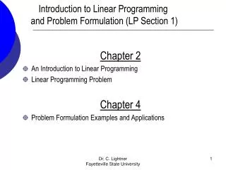
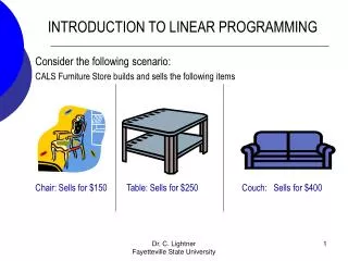
Chapter 2 Introduction to Linear Programming. Example of Linear Programming Problem. Each week the company can obtain: All needed raw material. Only 100 finishing hours. Only 80 carpentry hours. Also: Demand for the trains is unlimited.

E N D
Example of Linear Programming Problem • Each week the company can obtain: • All needed raw material. • Only 100 finishing hours. • Only 80 carpentry hours. • Also: • Demand for the trains is unlimited. • At most 40 soldiers are bought each week. Giapetto wants to maximize weekly profit (revenues – expenses). Formulate a mathematical model of Giapetto’s situation that can be used maximize weekly profit.
Example of Linear Programming Problem The Giapetto solution model incorporates the characteristics shared by all linear programming problems. x1 = # of soldiers produced each week x2 = # of trains produced each week Decision Variables Objective Function The decision maker wants to maximize (usually revenue or profit) or minimize (usually costs) some function of the decision variables.
Example of Linear Programming Problem Company’s weekly profit can be expressed in terms of the decision variables x1 and x2: Weekly profit = weekly revenue – weekly raw material costs – the weekly variable costs Weekly profit = (27x1 + 21x2) – (10x1 + 9x2) – (14x1 + 10x2 ) = 3x1 + 2x2
Example of Linear Programming Problem Constraint 1 Each week, no more than 100 hours of finishing time may be used. 2 x1 + x2≤ 100 Constraint 2 Each week, no more than 80 hours of carpentry time may be used. x1 + x2≤ 80 Constraint 3 Because of limited demand, at most 40 soldiers should be produced. x1≤ 40
Example of Linear Programming Problem The coefficients of the constraints are often called the technological coefficients. The number on the right-hand side of the constraint is called the constraint’s right-hand side (or rhs). Sign Restrictions If the decision variable can assume only nonnegative values, the sign restriction xi≥ 0 is added. If the variable can assume both positive and negative values, the decision variable xi is unrestricted in sign (often abbreviated urs).
Example of Linear Programming Problem optimization model: Max z = 3x1 + 2x2 (objective function) Subject to (s.t.) 2 x1 + x2≤ 100 (finishing constraint) x1 + x2≤ 80 (carpentry constraint) x1≤ 40 (constraint on demand for soldiers) x1≥ 0 (sign restriction) x2≥ 0 (sign restriction)
What Is a Linear Programming Problem? A linear programming problem (LP) is an optimization problem for which we do the following: • Attempt to maximize (or minimize) a linear function (called the objective function) of the decision variables. • The values of the decision variables must satisfy a set of constraints. • Each constraint must be a linear equation or inequality. • A sign restriction is associated with each variable. For each variable xi, the sign restriction specifies either that xi must be nonnegative (xi≥ 0) or that xi may be unrestricted in sign.
Assumptions of Linear Programming Proportionality and Additive Assumptions The objective function for an LP must be a linear function of the decision variables has two implications: 1. The contribution of the objective function from each decision variable is proportional to the value of the decision variable. 2. The contribution to the objective function for any variable is independent of the other decision variables.
Assumptions of Linear Programming Each LP constraint must be a linear inequality or linear equation has two implications: 1. The contribution of each variable to the left-hand side of each constraint is proportional to the value of the variable. 2. The contribution of a variable to the left-hand side of each constraint is independent of the values of the variable.
Assumptions of Linear Programming Divisibility Assumption The divisibility assumption requires that each decision variable be permitted to assume fractional values. The Certainty Assumption The certainty assumption is that each parameter (objective function coefficients, right-hand side, and technological coefficients) are known with certainty.
2.1 - What Is a Linear Programming Problem? The feasible region of an LP is the set of all points satisfying all the LP’s constraints and sign restrictions. Feasible Region and Optimal Solution • Give a point in feasible region • Give a point that is not in feasible region Giapetto Constraints 2 x1 + x2 ≤ 100 (finishing constraint) x1 + x2 ≤ 80 (carpentry constraint) x1 ≤ 40 (demand constraint) x1 ≥ 0 (sign restriction) x2 ≥ 0 (sign restriction)
What Is a Linear Programming Problem? For a maximization problem, an optimal solution to an LP is a point in the feasible region with the largest objective function value. Similarly, for a minimization problem, an optimal solution is a point in the feasible region with the smallest objective function value. Most LPs have only one optimal solution. However, some LPs have no optimal solution, and some LPs have an infinite number of solutions.
2.2 – Graphical Solution to a 2-Variable LP Since the Giapetto LP has two variables, it may be solved graphically. The feasible region is the set of all points satisfying the constraints: Finding the Feasible Solution Giapetto Constraints 2 x1 + x2 ≤ 100 (finishing constraint) x1 + x2 ≤ 80 (carpentry constraint) x1 ≤ 40 (demand constraint) x1 ≥ 0 (sign restriction) x2 ≥ 0 (sign restriction) A graph of the constraints and feasible region is shown on the next slide.
Graphical Solution to a 2-Variable LP Any point on or in the interior of the five sided polygon DGFEH(the shade area) is in the feasible region. Isoprofit line for maximization problem (Isocost line for minimization problem )is a set of points that have the same z-value
Two type of Constraints Binding and Nonbinding constraints A constraint is binding if the left-hand and right-hand side of the constraint are equal when the optimal values of the decision variables are substituted into the constraint.
Two type of Constraints A constraint is nonbinding if the left-hand side and the right-hand side of the constraint are unequal when the optimal values of the decision variables are substituted into the constraint.
Special Cases of Graphical Solution • Some LPs have an infinite number of solutions (alternative or multiple optimal solutions). • Some LPs have no feasible solution (infeasible LPs). • Some LPs are unbounded: There are points in the feasible region with arbitrarily large (in a maximization problem) z-values.
Alternative or Multiple Solutions Any point (solution) falling on line segment AE will yield an optimal solution with the same objective value
no feasible solution Some LPs have no solution. Consider the following formulation: No feasible region exists
Unbpunded LP The constraints are satisfied by all points bounded by the x2 axis and on or above AB and CD. There are points in the feasible region which will produce arbitrarily large z-values (unbounded LP).