Download
1 / 29
290 likes | 419 Views
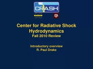
Center for Radiative Shock Hydrodynamics. Integration for Predictive Science R. Paul Drake. What lies ahead here. The CRASH process diagram, also with names Physical and computational models and studies Choice of models Related computational studies Validation

E N D
Center for Radiative Shock Hydrodynamics Integration for Predictive Science R. Paul Drake
What lies ahead here • The CRASH process diagram, also with names • Physical and computational models and studies • Choice of models • Related computational studies • Validation • The CRASH process in action • Initial discussion of some projects • Predictive simulation roadmap • Discussion of structure in the project • What we are doing to move this along Displaying bubble chart on other screen
The CRASH research process incorporates integrated UQ efforts. Culture change is here.
As requested, here is the distribution of our team across these activities (full table in handout)
The physical and numerical models p. 1 • Our approach to selection of physical models • If a correct local model exists, use it • Laser energy absorption coefficient • Thermal radiation emission rate • The justification for the local models is found in the CRASH Basics document • Ion-ion mean free path is always small • Electron-ion mean free path is always small • Electron heat flux is small save at obvious locations • Reynolds number is large everywhere Conduction 2D AMR test
The physical and numerical models p. 2 • Our approach to selection of physical models continued • In the few cases where no such model exists, use the best model that can be implemented and afforded and is legal • Flux-limited electron heat conduction • Multigroup diffusion radiative transfer • Laser energy deposition at critical density (small effect for CRASH problem) • A Laser Plasma Instability loss factor • Decisions to improve these models will be based on judgment in the face of experiments and predictions • For radiation transport specifically • Compare multigroup diffusion in CRASH-like systems with the SN model (PDT) we would have blithely implemented were we funded by NSF
The physical and numerical models p. 3 • Our approach to selection of physical models, continued • When known models are known to be significantly uncertain • This is only EOS and opacity • Implement physically consistent basic models that are well-suited for UQ (atomic-data based statistical physics approach) • Seek to compare these models with other models • We are funding collaborative work by Klapisch and Busquet on opacities and non-LTE effects • When choices must be made among numerical details • Assess performance for the range of physical processes that are of interest, including both fidelity and numerical errors • We document the associated choices • In the CRASH/BATSRUS manual • In the CRASH Basics reference document • In the CRASH UQ run set repository
Supporting computational efforts • We undertake computational projects • To address uncertainties in modeling of our primary system • As validation exercises (next slide) • Specific projects are discussed in posters • X-ray driven radiative shocks (Myra poster) • Pure hydro simulations (Fryxell poster) • X-ray driven low-Z walls (Drake poster) • Reverse radiative shock designs (Krauland poster) • Studies related to morphology (Powell talk) • NIF experiment (nothing new here) X-ray driven shock launched in Hyades CRASH
We are pursuing validation • Validation occurs in various ways • Modeling of a variety of physical systems • Helps establish and expand the physical regimes we can model • Detailed comparison with specific experiments • We have the data for validation of various components and are pursing some validation efforts • This often needs to take a back seat to the main project and to verification and debugging • In choosing new experiments, we pursue those issues most critical to our ultimate predictive study • Current plans • Early time data (this year) • Do final experiment in year 4 and repeat in year 5
The laser interaction phase (for either code) • We go through the entire process to calibrate • Responsibilities (Team leads in parentheses) • Laser software • Applications team (Drake) for Hyades cases • Code team (Powell) for CRASH laser software • Done by Sokolov and Torralva with Van derHolst • Experiments team (Drake) for measurements • Applications team (Drake) for large run sets • Fryxell or Grosskopf lead in various cases • UQ team (Holloway) for run-set design and post-run-set calibration • flux limiter; laser energy Hyades grid
Our predictive study with calibration was an integrated effort (details in Holloway talk later) • Selected variables and run-set design, did Hyades run set • Calibration step • We did a CRASH 2.0 run set fed by the Hyades output • We extracted metrics (shock location, interface location) • We analyzed the results (a UQ process) to predict these metrics at a much later observation time (26 ns) • We made such measurements • Obtained data at 20 and 26 ns • Comparison to be unveiled this afternoon We also did a calibrated predictive study from the H2D run set (Stripling Poster)
A key element in any run set is deciding that the code output makes physical sense • It would be completely wrong to leave one’s brain outside the door when proceeding to do UQ • Need to check and to test suspicious results • An important consequence is finding bugs • This need, to thoughtfully examine the output, will be and should be a rate-limiting factor in all our predictive studies • Not having plausible multi-D behavior, we decided to do 1D predictive science studies that developed new methods • This is what we did this past year Spring 2010 Hyades Spring 2010 CRASH Now (Fall 2010) appear to be ready to move more quickly with CRASH
The current experimental thrust is early post-laser data • We began with no constraints, considering every experiment we could think of • We came to realize that the physically tricky early period is probably key in establishing the shock morphology • Early simultaneous blowoff over some distance • Later development of tilted wall shock • Complex simulated morphology limits the accuracy of our predictions and the precision of viable metrics • Led to decision to seek early time and multi-frame data Log density at 4.5 ns shows shock structure
We are putting in place the pieces to enable more rapid and multi-D UQ studies • Escaping Hyades (but not free yet) • Using integrated metrics • Positioning more people to do CRASH runs • Positioning more people to run UQ software Automated analysis of 104 runs – details in Holloway talk
The year 4/5 experiment study is a challenge • Necessarily 3D • Need pdfs corresponding to laser interactions to start • H2D problems are limiting element • Need viable metrics that function with simulation output • Went to integrated metrics • Need non-pathological morphologies • Required sufficiently debugged CRASH 2 • Seem to be there now, however • First need study in support of approaching year 3 experiment • Computational limitations imply that the year 4/5 study must combine models having different levels of fidelity • 2D multigroup and 3D gray will be more numerous than well-resolved 3D runs
Looking ahead • We are ready for multi-D integrated studies • The major constraint appears to be computational resources • Opportunities for future evolution toward and beyond year 5 • Extensive engagement of uncertainty across model fidelity • Radtran model • Dimensionality • Resolution • Inconsistency across more sophisticated EOS and opacity models • Treatment of heat conduction in laser absorption • Facing model calibration with multiple measurements • X-ray Thomson Scattering will soon provide quantification of temperature profiles
Minimal CRASH needs to predict year 4/5 • Electron Flux Limiter • LSF (1D Hyades initialization) • Laser Energy • Be Thickness • Tube Radius • Xe Fill Pressure • Backlighter Fire Time • Nozzle Angle • Plenum Length • Tube Radius (post nozzle) • Aspect Ratio (3D only) • At least 2^10 = 1024 runs of “worst” model (2D-G) (Orthogonal LHD) • 512 runs of 2DMG (compare ½ of 2D-G with 2D-MG) • 256 runs of 3D-G (compare ¼ of 2D-G with 3D-G and ½ of 2D-MG with 3D-G) • 256 3D-MG medium resolution runs • 8 - 16 3D-MG high res runs (or what we discover we can afford) • Determine best aspect ratios (will be very sparse in 11D) • Preferable to at least double all these numbers • Smallest recommended LHD over 11D = 2048
Runsets (RS) • RS1: 320 pts in 8D 1D Hyades & Crash • RS2: 512 pts in 15D 1D Hyades • RS3: 1024 pts in 6D 1D Hyades & Crash • RS4: 104 pts in 5D 2D Hyades • RS5: Nov 2010 1D convergence study (512 1D-MG) • RS6: Nov 2010 2D convergence study (128 2D-MG) • RS7: Nov 2010 Sensitivity Study (256 runs 2D G & MG) • RS8: Early 2011 2D nozzle study with large tubes (128 2D runs) • RS9: Early 2011 3D aspect ratio sensitivity study (256 runs 3D-G) • RS10: Early 2011 Full simulation with 2D-G 1024 runs • RS11: 2011 Full simulation with 2D-MG 512 runs • RS12: 2011 Full simulation with 3D-G 256 runs • RS13 : 2011 Full simulation with 3D-MG 8-16 runs
RS 5 & 6: 2010 convergence • Outputs: • Shock Location • Axial Centriod • Area of dense Xe • Radial Mean (zero in 2D) • Radial Mean sq. • 512 runs for 1D • 128 runs for 2D (32 min) • Inputs: • Grid resolution (600 – 38400 1D) • Groups (10 – 90) • Lower Freq (0.1 – 1 eV) • Upper Freq (1 – 10 keV) • Table resolution (1002 – 6002) • Fixed backlighter time 12 ns • 1D Hyades uses CRASH EOS, Single Hyades run for initialization, using radiation temp only
RS 7: 2010 sensitivity study • Outputs: • SL • AC • Area • Radial mean • Radial mean sq. • 128 runs each of: • 2D-G • 2D-MG • Inputs: • EFL • LSF • Laser Energy • Be thickness • Xe fill pressure • Backlighter time • Tube radius
RS 8: 2D Nozzle study with large tubes • Outputs: • SL • AC • Area • Radial mean • Radial mean sq. • 64 runs each of: • 2D-G • 2D-MG • Inputs: • EFL • LSF • Laser Energy • Be thickness • Xe fill pressure • Tube radius • Fixed backlighter time ?? ns
RS 9: 3D aspect ratio sensitivity study • Outputs: • SL • AC • Area • Radial mean • Radial mean sq. • Both measured in 2 views • 128 runs each of: • 3D-G • 3D-MG(moderate resolution) • A few 3D-MG (high res) • Inputs: • EFL • Laser energy • Be thickness • Xe fill pressure • Tube radius • Aspect ratio • Grid resolution of ellipse • Fixed backlighter time • Initialized from H2D large tube runs
RS 10/11: Full simulation with 2D-G/MG 1024 runs • Outputs: • SL • AC • Area • Radial mean • Radial mean sq. • 1024 runs of 2D-G • 512 runs of 2D-MG • Inputs: • Electron flux limiter • LSF (1D Hyades initialization) • Laser Energy • Be Thickness • Tube Radius • Xe Fill pressure • Backlighter fire time • Nozzle angle • Nozzle length • Tube radius (post nozzle)
RS 12: Full simulation with 3D-G 256 runs • Outputs: • SL • AC • Area • Radial mean • Radial mean sq. • 256 runs of 3D-G • Inputs: • Electron flux limiter • LSF (1D Hyades initialization) • Laser Energy • Be Thickness • Tube Radius • Xe Fill pressure • Backlighter fire time • Nozzle angle • Nozzle length • Tube radius (post nozzle) • Aspect ratio
RS 13: Full simulation with 3D-MG runs • Outputs: • SL • AC • Area • Radial mean • Radial mean sq. • 8-16 runs of 3D-MG or whatever we can afford • Inputs: • Electron flux limiter • LSF (1D Hyades initialization) • Laser Energy • Be Thickness • Tube Radius • Xe Fill pressure • Backlighter fire time • Nozzle angle • Nozzle length • Tube radius (post nozzle) • Aspect ratio