Download
1 / 39
390 likes | 474 Views
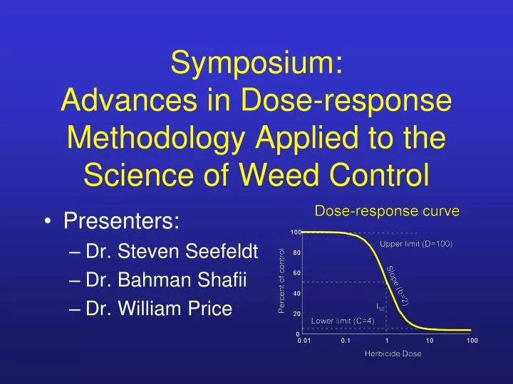
Symposium: Advances in Dose-response Methodology Applied to the Science of Weed Control. Presenters: Dr. Steven Seefeldt Dr. Bahman Shafii Dr. William Price. Historical development of dose-response relationships. Steven Seefeldt, ARS, Fairbanks, AK Bahman Shafii, Univ. of ID, Moscow, ID

E N D
Symposium: Advances in Dose-response Methodology Applied to the Science of Weed Control • Presenters: • Dr. Steven Seefeldt • Dr. Bahman Shafii • Dr. William Price
Historical development of dose-response relationships Steven Seefeldt, ARS, Fairbanks, AK Bahman Shafii, Univ. of ID, Moscow, ID William Price, Univ. of ID, Moscow, ID
What did hunter gathers do? One Several Dinner Tasty Tasty Filling
What did hunter gathers do? One Several Dinner Tasty Tasty Filling Tasty Tasty Stomach ache
What did hunter gathers do? One Several Dinner Tasty Tasty Filling Tasty Tasty Stomach ache Stomach Dead Still Dead ache
Response curve Assumptions: 1. Small dose increases at some threshold result in very large responses and 2. susceptibility to dose is normally distributed
Linear regression Initially can determine least squares, but is it useful for estimating anything other than dose resulting in 50 % response?
Remember least squares? With 4 bivariate options Sums of Squares X=10/4=2.5 Y=9/4=2.25 b=(25-4(2.5)(2.25))/((30-(4(2.5) 2)=0.5 a=2.25-0.5(2.5)=1 Line equation is y=1 + 0.5x R2 = 1-ESS/TSS=1-(1.5/2.75)=0.455
Early work on response curves • Pearl and Reed. 1920. Proceed. Nat. Acad. of Sci. V6#6:275-288. • Mathematical representation of US population growth. • Improved on Pritchett’s 1891 model (a third order parabola) on US population growth. • Made it binomial and logarithmic (y = a + bx + cx2 + d log x)
Early work on response curves • They recognized that equation would not predict US population into the future so, assuming that resources would limit populations, they postulated: • y = b/(e-ax + c) for x > 0, y = b/c • point of inflection is x = -(1/a)log e and y = b/2c • slope at point of inflection is ab/4c
Early work on response curves • They recognized that equation would not predict US population into the future so, assuming that resources would limit populations, they postulated: • y = b/(e-ax + c) for x > 0, y = b/c • point of inflection is x = -(1/a)log e and y = b/2c • slope at point of inflection is ab/4c • Their inflection point was April 1, 1914 at a population of 98,637,000 and a population limit of 197,274,000
Early work on response curves • They recognized that equation would not predict US population into the future so, assuming that resources would limit populations, they postulated: • y = b/(e-ax + c) for x > 0, y = b/c • point of inflection is x = -(1/a)log e and y = b/2c • slope at point of inflection is ab/4c • Their inflection point was April 1, 1914 at a population of 98,637,000 and a population limit of 197,274,000 • They recognized 2 problems • Location of the point of inflection • Symmetry
Early work on response curves • Pearl in 1927 published “The Biology of Superiority”, which disproved basic assumptions of eugenics and went on to a career in Mendelian genetics. • Reed in 1926 became the second chair of Biostatistics at John Hopkins and by 1953 was president of the university.
Early work on response curves • Pearl in 1927 published “The Biology of Superiority”, which disproved basic assumptions of eugenics and went on to a career in Mendelian genetics. • Reed in 1926 became the second chair of Biostatistics at John Hopkins and by 1953 was president of the university. • In 1929 Reed and Joseph Berkson published “The Application of the Logistic Function to Experimental Data” in an attempt to correct rampant misuse. • “in almost all cases, the mathematical phases of the treatment have been faulty, with consequent cost to precision and validity of the conclusions”
Early work on response curves • They made the recommendation that this curve be referred to as logistic instead of autocatalytic because the curve was being used where “the concept of autocatalysis has no place”.
Early work on response curves • They made the recommendation that this curve be referred to as logistic instead of autocatalytic because the curve was being used where “the concept of autocatalysis has no place”. • Later they state that “the method of least squares, when certain assumptions regarding the distribution of errors can be made, is mathematically the most proper”.
Early work on response curves • They made the recommendation that this curve be referred to as logistic instead of autocatalytic because the curve was being used where “the concept of autocatalysis has no place”. • Later they state that “the method of least squares, when certain assumptions regarding the distribution of errors can be made, is mathematically the most proper”. • After acknowledging the computational difficulties, they consider other techniques to determine the parameters: Logarithmic Graphic Method; Function of (r, y, t) vs. y; Slope of the Logarithmic Function vs. y; and Parameters of the Hyperbola.
Early work on response curves • All these methods involved graphing, fitting a line by eye, and in some cases changing the multiplier and repeating the process until better linearity results. • They note that “One attempts in doing this to choose a line that minimizes the total deviations.” and that “The inexactness that might appear in such a method is not as serious as sometimes supposed” • Also, “Hand calculations of non-linear statistical estimations are labor intensive and prone to error” • And “Iterative procedures result in greater expenditures for labor and more opportunities for calculation error”
Working with a transformation • Once the line was drawn (fitted) through the data points the slope (2.30259 x m) and intercept (log-1 a) are determined (Reed and Berkson 1929) • Expected and observed outcomes could then be compared.
More linear transformations • Integral of the normal curve (Gaddum 1933) • Widely used to represent the distribution of biological traits • Direct experimental evidence for a normal distribution of susceptibility (tolerance distribution) • Gaddum was an English pharmacologist who wrote classic text Gaddum's Pharmacology
More linear transformations • Probit (C. I. Bliss 1934) • Observation that in many physiologic processes equal increments in response are produced when dose is increased by a constant proportion of the given dosage, rather than by constant amount. • Chester Bliss was largely self • Taught, worked with Fisher, and • eventually settled at Yale.
Working with a transformation • Tables with transformations were prepared
More linear transformations • Logistic function applied to bioassy (Berkson 1944) and ED50 • Biologically relevant • Autocatalysis of ethyl acetate by acetic acid • Oxidation-reduction reaction • Bimolecular reaction of methyl bromide and sodium thiosulfate • Hydrolysis of sucrose by invertase • Hemolysis of erythrocytes by NaOH
More linear transformations • Logistic function applied to bioassy (Berkson 1944) and ED50 • Biologically relevant • Autocatalysis of ethyl acetate by acetic acid • Oxidation-reduction reaction • Bimolecular reaction of methyl bromide and sodium thiosulfate • Hydrolysis of sucrose by invertase • Hemolysis of erythrocytes by NaOH • Berkson of the Mayo clinic sadly stated in 1957 that it was “very doubtful that smoking causes cancer of the lung”
Working with a transformation • Special graph paper was designed
Statistical analyses • Least squares vs Maximum likelihood • Berkson (1956) revived the debate started by Fisher in 1922. • Because of lack of computational power the point was all but moot • There was general agreement that maximum likelihood was best
Computers • By 1990, increased computational speed and accuracy and the development of analysis software meant that analyses of dose-response relationships could be conducted using iterative least squares estimation procedures
Early dose-response, a primer • Preliminary ANOVA • Logistic equation • Dose-response curve • Treatment comparison • Model comparison • Practical use
Preliminary ANOVA • Determines if herbicide dose has an effect on plant response • Provides the basis for a lack-of-fit test of the subsequent nonlinear analysis • Provides the basis for assessing the potential transformation of response variables
Log-logisitic equation D-C y=C+ 1+exp[b(log(x)-log(I ))] 50 D = Upper limit C = Lower limit b = Related to slope I = Dose giving 50% response 50 Seefeldt et al. 1995
Log transformation of dose More or less symmetric sigmoidal curve that expands the critical dose range where response occurs
Dose-response curve 100 Upper limit (D=100) 80 60 Percent of control Slope (b=2) 40 I50 20 Lower limit (C=4) 0 0.01 0.1 1 10 100 Herbicide Dose
Treatment comparison 100 Upper limit (D=100) 80 60 Percent of control Slope (b=2) 40 I50 I50 20 Lower limit (C=4) 0 0.01 0.1 1 10 100 Herbicide Dose
Treatment comparison 100 Upper limit (D=100) 80 60 Slope (b=1.2) Percent of control Slope (b=2) 40 I50 I50 20 Lower limit (C=4) 0 0.01 0.1 1 10 100 Herbicide Dose
Comparing crop (pale blue) to weed (yellow) 100 I5 80 60 Percent of control 40 I95 20 0 0.01 0.1 1 10 100 Herbicide Dose
Usefulness • Biologically meaningful parameters • Least squares summary statistics • Confidence intervals • Better estimates of response at high and low doses • Tests for differences in I50 or slope • Still errors at extremes of doses
References • Bliss, C. I. 1934. The method of probits. Science, 79:2037, 38-39. • Berkson, J. 1944. Application of the Logistic function to bio-assay. J. Amer. Stat. Assoc. 39: 357-65. • Berkson, J. 1955. Estimation by least squares and by maximum likelihood. Third Berkeley Symposium p1-11. • Gaddum, J. H. 1933. Methods of biological assay depending on a Quantal response. Medical Res. Council Special Report. Series No. 183. • Reed, L.J., and Berkson, J. 1929. The application of the logistic function to experimental data. J. Physical Chem. 33:760-779. • Seefeldt, S.S., J. E. Jensen, and P. Fuerst. 1995. Log-logistic analysis of herbicide dose-response relationships. Weed Technol. 9:218-227.