Download
1 / 28
280 likes | 429 Views
Lesson overview. Chapter 5 Simultaneous Move Games with Pure Strategies … Lesson I.8 Simultaneous and Continuous Move Theory Each Example Game Introduces some Game Theory Example 1: Continuous Variables Example 2: Risk in Nash Equilibrium Example 3: Rationality in Nash Equilibrium

E N D
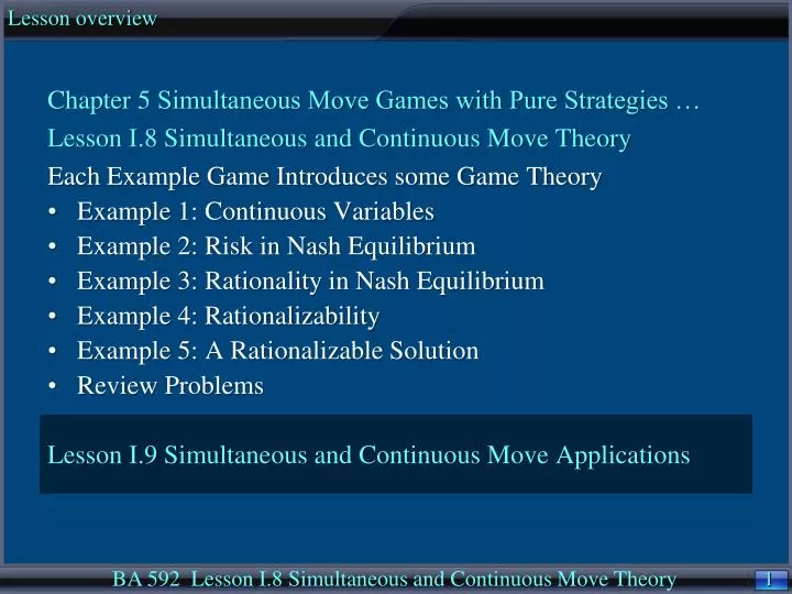
Lesson overview • Chapter 5 Simultaneous Move Games with Pure Strategies … • Lesson I.8 Simultaneous and Continuous Move Theory • Each Example Game Introduces some Game Theory • Example 1: Continuous Variables • Example 2: Risk in Nash Equilibrium • Example 3: Rationality in Nash Equilibrium • Example 4: Rationalizability • Example 5: A Rationalizable Solution • Review Problems • Lesson I.9 Simultaneous and Continuous Move Applications BA 592 Lesson I.8 Simultaneous and Continuous Move Theory
Example 1: Continuous Variables Best-response analysis for finding all the Nash equilibria of simultaneous-move games can be extended from games with a finite number of available strategies to a continuum of strategies. To calculate best responses in this type of game, we find, for each possible value of one player’s strategy, the value of the other player’s strategy that is best for it. The continuity of the sets of strategies allows us to use algebraic formulas to show the best responses as curves in a graph, with each player’s strategy on one of the axes. The Nash equilibrium of the game is where the two curves meet. BA 592 Lesson I.8 Simultaneous and Continuous Move Theory
Example 1: Continuous Variables Walmart and Costco compete on price to sell some goods that are perfect substitutes(like emergency food supplies in a weather-proof bucket), while other goods are imperfect substitutes (like prepared pizzas). Suppose Walmart sets the price Px of their good at the same time Costco sets the price Py of their good. And suppose, given these prices, demands are Qx = 44 -2 Px + Py Qy = 44 -2 Py + Px (The terms + Pyand + Pxindicate the goods are substitutes --- better gross substitutes.) And suppose unit supply costs are $8. Compute best-response curves for this Price Competition Game, then intersect the curves to find the Nash equilibria. Can the two firms each increase profit if they can commit to different strategies? BA 592 Lesson I.8 Simultaneous and Continuous Move Theory
Example 1: Continuous Variables Given prices Px and Py of the two goods, use demand and cost to compute profits: Px = (Px- 8) Qx = (Px- 8)(44 -2 Px + Py) = - 8(44 + Py) + (60 + Py)Px – 2(Px)2 Py = (Py- 8) Qy = (Py- 8)(44 -2 Py + Px) = - 8(44 + Px) + (60 + Px)Py – 2(Py)2 Since Px is a concave function of PxandPy is a concave function of Py, profits Px(Px) and Py(Py) are maximized where their derivatives are zero. 0 = Px’(Px) = (60 + Py) – 4Px 0 = Py’(Py) = (60 + Px) – 4Py BA 592 Lesson I.8 Simultaneous and Continuous Move Theory
Example 1: Continuous Variables Best-response curves for the Price Competition Game are the solutions to those first-order conditions: 0 = (60 + Py) – 4Px 0 = (60 + Px) – 4Py meaning solve the first equation for best-response curve Px = 15 + .25Py and the second equation for best-response curve for Py = 15 + .25Px Substituting the first curve into the second yields Py = 15 + .25(15 + .25Py) = 18.75 + 0.0625 Py and the unique solution Py = 20. Hence, the first curve yields Px = 15 + .25(20) = 20. The Nash equilibrium is thus (Px,Py) = (20,20). BA 592 Lesson I.8 Simultaneous and Continuous Move Theory
Example 1: Continuous Variables Can the two firms each increase profit if they can commit to different strategies? At (Px,Py) = (20,20), Px = (Px– 8) Qx = (Px– 8)(44 – 2 Px + Py) = 12(24) = 288 Py = (Py– 8) Qy = (Py– 8)(44 – 2 Py + Px) = 12(24) = 288 But at non-equilibrium prices (Px,Py) = (P,P), Px = (Px– 8) Qx = (P– 8)(44 – 2 P + P) = – 352 + 52P – P2 Py = (Py– 8) Qy = (P– 8)(44 – 2 P + P) = – 352 + 52P – P2 Since Px andPy are a concave function of P, profits Px(P) and Py(P) are maximized where their derivatives are zero: 0 = Px’(P) = 52 – 2P and 0 = Py’(P) = 52 – 2P, so P = 26. The two firms each increase profit if they can commit to increase price from P = 20 to P = 26. BA 592 Lesson I.8 Simultaneous and Continuous Move Theory
Example 2: Risk in Nash Equilibrium Risk neutral players’ evaluate uncertain outcomes by their expected value. For example, if payoffs in a game are in dollars, then a risk-neutral player would be indifferent between being given $10 and flipping a coin for double or nothing. Later lessons accommodate risk averse players (even risk loving players), but for now consider just the simplest case of risk neutral players. BA 592 Lesson I.8 Simultaneous and Continuous Move Theory
Example 2: Risk in Nash Equilibrium What strategy should Walmart choose in the following game with Costco? There is only one Nash Equilibrium:Walmart chooses A and believes Costco chooses A. Is that that Nash equilibrium a reasonable recommendation? Objection: Is not C better because it guarantees the Nash equilibrium outcome of 2? BA 592 Lesson I.8 Simultaneous and Continuous Move Theory
Example 2: Risk in Nash Equilibrium Objection: Is not C better because it guarantees the Nash equilibrium outcome of 2? Response: Not necessarily. The Nash equilibrium recommendation of A is appropriate when you absolutely believe the other player also chooses A. The guaranteed payoff from C is only relevant if your belief is not absolute but, rather, there is a probability 1-p-q<1 that Costco chooses A, a small probability p>0 that Costco chooses B, and a small probability q>0 that Costco chooses C. Given those non-absolute beliefs, Walmart thus expects payoff 2(1-p-q) + 3p from A, which is larger (A is better) than the guaranteed payoff of 2 from C when 2(-p-q)+3p > 0, or p-2q > 0. BA 592 Lesson I.8 Simultaneous and Continuous Move Theory
Example 2: Risk in Nash Equilibrium What strategy should Walmart choose in the following game with Costco? There is only one Nash Equilibrium:Walmart chooses Down and believes Costco chooses Left. Is that that Nash equilibrium a reasonable recommendation? Objection: Is not Up better because it avoids the possibility of loosing 1000? BA 592 Lesson I.8 Simultaneous and Continuous Move Theory
Example 2: Risk in Nash Equilibrium Objection: Is not Up better because it avoids the possibility of loosing 1000? Response: Not necessarily. The Nash equilibrium recommendation of Down is appropriate when you absolutely believe the other player chooses Left. The safer payoff from Up is only relevant if your belief is not absolute but, rather, there is a probability 1-p<1 that Costco chooses Left and a small probability p>0 that Costco chooses Right. Given those non-absolute beliefs, Walmart thus expects payoff 10(1-p) - 1000p from Up, which is larger (Down is better) than the safer expected payoff of 9(1-p) + 8p from Up when 10(1-p) - 1000p > 9(1-p) + 8p, or p < 1/1019. BA 592 Lesson I.8 Simultaneous and Continuous Move Theory
Example 2: Risk in Nash Equilibrium Objection: Would you risk the possibility of loosing $1000 for a gain of $1? Response: Have you ever driven at a higher speed (risking more than $1000 if you get in an accident) to save a few minutes and so gain $1 of time, which you could spend at work or spend at home looking for a lost pack or gum or a lost battery so you do not have to spend $1 to replace it. To dispel any doubt, the European Road Safety Observatory says a higher speed increases the likelihood of an accident. Very strong relationships have been established between speed and accident risk: The general relationship holds for all speeds and all roads, …. BA 592 Lesson I.8 Simultaneous and Continuous Move Theory
Example 3: Rationality in Nash Equilibrium What strategy should Sam’s Club choose in the following game with Costco? There is only one Nash Equilibrium: (R2,C2). Is that the only reasonable recommendation? BA 592 Lesson I.8 Simultaneous and Continuous Move Theory
Example 3: Rationality in Nash Equilibrium There is only one Nash Equilibrium: (R2,C2). Is that the only reasonable recommendation? Some claim it is. Sam’s plays R2 because Sam’s believes Costco will play C2. And why does Sam’s believe this? Because Sam’s believes Costco to be rational, Sam’s must believe that Costco believes that Sam’s is choosing R2, because C2 would not be Costco’s best choice if Costco believed Sam’s would choose either R1 or R3. Thus, some claim, in any rational process of formation of beliefs and responses, Sam’s would only choose a strategy that is part of a Nash equilibrium, where beliefs are correct. But that argument stops after one round of thinking about beliefs. BA 592 Lesson I.8 Simultaneous and Continuous Move Theory
Example 3: Rationality in Nash Equilibrium R2 is, in fact, not the only reasonable recommendation for Sam’s. R1 is reasonable if Sam’s believes that Costco will choose C3, which Costco will choose if Costco believes that Sam’s will choose R3, which Sam’s will choose if Sam’s believes that Costco will choose C1, which Costco will choose if Costco believes that Sam’s will choose R1, and so on. Likewise, R3 is reasonable if Sam’s believes that Costco will choose C1, which Costco will choose if Costco believes that Sam’s will choose R1, and so on. BA 592 Lesson I.8 Simultaneous and Continuous Move Theory
Example 4: Rationalizability What strategy should Row choose in the following game with Column? R1 is reasonable if R believes C will choose C3, which C will choose if C believes R will choose R3, which R will choose if R believes C will choose C1, which C will choose if C believes R will choose R1, and so on. BA 592 Lesson I.8 Simultaneous and Continuous Move Theory
Example 4: Rationalizability R2 is reasonable if R believes C will choose C2, which C will choose if C believes R will choose R2, and so on. R3 is reasonable if R believes C will choose C1, which C will choose if C believes R will choose R1, which R will choose if R believes C will choose C3, which C will choose if C believes R will choose R3, and so on. R4 is never reasonable no matter what R believes C will choose. R1, R2, and R3 are thus Rationalizeable. But R4 is not, even though R4 is not (strictly or weakly) dominated by any other row. BA 592 Lesson I.8 Simultaneous and Continuous Move Theory
Example 5: A Rationalizability Test Rationalizability is confirmed when you hit a cycle, and you can find all in this way when there is only a finite number of strategies. To cover continuous moves, rationalizability test is the iterated elimination of strategies that are not the best response to any strategies by the other players. BA 592 Lesson I.8 Simultaneous and Continuous Move Theory
Example 5: A Rationalizability Test Gloucester Massachusetts has two fishing boats the go out every evening and return the following morning to bring their night’s catch to the market. All fish has to be sold and eaten the same day. Fish are plentiful, so each boat decides how many fish to bring to the market. But each knows that, if the total that is brought to the market is too large, the glut of fish means low prices and low profits. Suppose the price of fish is P = 60 – (G+M) if George Clooney’s boat brings back G barrels and Mark Wahlberg’s boat brings back M barrels. Suppose unit costs of production are 30 for George, and 36 for Mark. Find all rationalizable strategies for this Quantity Competition (Cournot) Game. BA 592 Lesson I.8 Simultaneous and Continuous Move Theory
Example 5: A Rationalizability Test Given quantities G and M of the two boats, use price and cost to compute profits: PG = ((60-G-M)-30)G = (30– M)G – G2 PM = ((60-G-M)-36)M = (24– G)M – M2 Since PG is a concave function of Gand PM is a concave function of M, profits PG(G) and PM(M) are maximized where their derivatives are zero. 0 = PG’(G) = (30– M) – 2G, or G = 15 – M/2 0 = PM’(M) = (24– G) – 2M, or M = 12 – G/2 BA 592 Lesson I.8 Simultaneous and Continuous Move Theory
Example 5: A Rationalizability Test Use the best response curves G = 15 – M/2 and M = 12 – G/2. BA 592 Lesson I.8 Simultaneous and Continuous Move Theory
Example 5: A Rationalizability Test First round of eliminations, only G in the closed interval [0,15] is a best response to some M, and only M in the closed interval [0,12] is a best response to some G. BA 592 Lesson I.8 Simultaneous and Continuous Move Theory
Example 5: A Rationalizability Test Second round of eliminations, only G in [9,15] is a best response to some M in [0,12], and only M in [4.5,12] is a best response to some G in [0,15]. BA 592 Lesson I.8 Simultaneous and Continuous Move Theory
Example 5: A Rationalizability Test Third round of eliminations, only G in [9,12.75] is a best response to some M in [4.5,12], and only M in [4.5,7.5] is a best response to some G in [9,15]. BA 592 Lesson I.8 Simultaneous and Continuous Move Theory
Example 5: A Rationalizability Test Fourth round of eliminations, only G in [11.25,12.75] is a best response to some M in [4.5,7.5], and only M in [5.625,7.5] is a best response to some G in [11.25,12.75]. BA 592 Lesson I.8 Simultaneous and Continuous Move Theory
Example 5: A Rationalizability Test Fifth round of eliminations, only C in [11.25,12.1875] is a best response to some M in [5.625,7.5], and only M in [5.625,6.375] is a best response to some C in [11.25,12.75]. BA 592 Lesson I.8 Simultaneous and Continuous Move Theory
Example 5: A Rationalizability Test And so on as the intervals converge to a single point, which is the Nash equilibrium solution (G,M) = (12,6) to the best-response curves G = 15 – M/2 and M = 12 – G/2. Therefore, (G,M) = (12,6) are the unique rationalizeable strategies. BA 592 Lesson I.8 Simultaneous and Continuous Move Theory
BA 592 Game Theory End of Lesson I.8 BA 592 Lesson I.8 Simultaneous and Continuous Move Theory