Download
1 / 38
380 likes | 619 Views
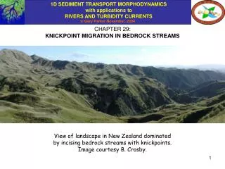
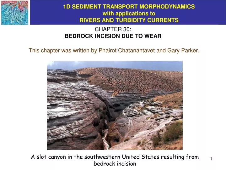
CHAPTER 30: BEDROCK INCISION DUE TO WEAR. This chapter was written by Phairot Chatanantavet and Gary Parker. A slot canyon in the southwestern United States resulting from bedrock incision. FROM m&n’s TO A MORE PHYSICALLY-BASED MODEL OF BEDROCK INCISION.

E N D
CHAPTER 30: BEDROCK INCISION DUE TO WEAR This chapter was written by Phairot Chatanantavet and Gary Parker. A slot canyon in the southwestern United States resulting from bedrock incision
FROM m&n’s TO A MORE PHYSICALLY-BASED MODEL OF BEDROCK INCISION In Chapter 16: Morphodynamics of Bedrock-alluvial Transitions, it is assumed that the bedrock platform is fixed in time and is not free to undergo incision. This is generally true at the scale of adjustment of alluvial streams, but is not true in longer geomorphic time. In Chapter 29: Knickpoint Migration in Bedrock Streams, a formulation for the morphodynamics of bedrock streams was developed using the following incision law: This relation has provided useful results, but does not adequately express the physics of the incisional process. Recently Parker (2004) has developed a model that incorporates three mechanisms: a) wear caused as bedload particles strike bedrock (Sklar and Dietrich, 2004), plucking, by which chunks of fractured bedrock are torqued out of the bed by the flow and broken up, and macroabrasion, by which these chunks are further broken up as bedload particles strike them (Whipple et al., 2000). Here a model of incision due to wear based on Sklar and Dietrich (2004) is developed.
OVERVIEW OF BEDROCK INCISION As noted in the previous slide, aspects of bedrock rivers were introduced in Chapter 16 and 29. As described in Chapter 16, a bedrock river has patches of bed that are not covered by alluvium, and where bedrock is exposed. There are many ways to cause a river to incise into its own bedrock. In this chapter, only the process of wear (abrasion) is considered (e.g. Sklar and Dietrich, 2004). That is, the bedrock is gradually worn away as bedrock particles strike regions of the bed where bedrock is exposed. A bedrock river in Kentucky (tributary of Wilson Creek) with a partial alluvial covering. Image courtesy A. Parola. A bedrock river in Japan. Image courtesy H. Ikeda.
BEDROCK INCISIONAL ZONE Floor of subsiding graben Alluvial fan Uplifting, incising zone Incisional zone and alluvial fan in Tarim Basin, China. Bedrock incision does not need to, but can be strongly driven by uplift. The Above example shows incision in an uplifting mountain zone, with the resulting sediment deposited in an adjacent subsiding graben.
HILLSLOPE DIFFUSION AND LANDSLIDING Oregon Coast Range USA, Image courtesy Bill Dietrich As the channel cuts down in response to uplift, it causes the adjacent hillslopes to erode by hillslope diffusion or landsliding.
WEAR (ABRASION) PROCESS DRIVEN BY COLLISION The model for incision driven by wear presented here is similar to that given in Sklar and Dietrich (2004). Wear or abrasion is the process by which stones colliding with the bed grind away the bedrock to sand or silt. Wear is treated in terms of relations of the same status as those used to predict gravel abrasion in rivers (e.g. Parker, 1991). The stones that do the wear are assumed to have a characteristic size Dw. Let q(x) denote the volume transport rate of sediment in the stream per unit width (L2/T) during the storm events that drive abrasion. Let the fraction of this load that consists of particles coarse enough to do the wear be . The volume transport rate per unit width qwear of sediment coarse enough to wear the bedrock is then given as
WEAR PROCESS DRIVEN BY COLLISION contd. For simplicity, might be set equal to the fraction of the load that is gravel or coarser. A more sophisticated formulation might use a discriminator such as the ratio of shear velocity to fall velocity, as in Sklar and Dietrich (2004). Here is taken to be a prescribed constant. Consider the case of saltating bedload particles. Let Esaltw denote the volume rate at which saltating wear particles bounce off the bed per unit bed area [L/T] and Lsaltw denote the characteristic saltation length of wear particles [L]. It follows from simple continuity that The mean number of bed strikes by wear particles per unit bed area per unit time is equal to Esaltw/Vw, where Vw denotes the volume of a wear particle. It is assumed that with each collision a fraction r of the particle volume is ground off the bed (and a commensurate, but not necessary equal amount is ground off the wear particle). The rate of bed incision vIw due to wear is then given as (number of strikes per unit bed area) x (volume removed per unit strike), or
WEAR PROCESS DRIVEN BY COLLISION contd. from and It is found that Here the parameter w has dimensions [1/L], and has exactly the same status as the abrasion coefficients used to study downstream fining by abrasion in rivers. This parameter could be treated as a constant. In so far as Lsaltw depends on flow conditions and r depends on rock type and perhaps the strength of the collision, w might be expected to vary somewhat with flow and lithology. The above relation is valid only to the extent that all wear particles collide with exposed bedrock. If wear particles partially cover the bed, the wear rate should be commensurately reduced. This effect can be quantified in terms of the ratio qwear/qwearc, where qwearc denotes the capacity transport rate of wear particles. Let po denote the areal fraction of surface bedrock that is not covered with sediment. In general po can be expected to approach unity as qwear/qwearc 0, and approach zero as qwear/qwearc 1.
COVER FACTOR FOR INCISION BY WEAR A “cover function” of the following type is proposed by Sklar and Dietrich (2004); , therefore and finally Wear particles striking other wear particles do not wear the bed qwear/qwearc Note that vIw drops to zero when q becomes equal to qwearc, downstream of which a completely alluvial gravel-bed stream is found. That is, the above formulation can describe the end point of the incisional zone as well as the incision rate.
EXPERIMENT ON UNDERCAPACITY TRANSPORT OF GRAVEL The image on the left shows an inerodible concrete- bed flume with grooves at St. Anthony Falls Laboratory, University of Minnesota, USA. The design of the grooves is based on Piccaninny Creek, Australia (Wohl, 1998). Experiments are underway to investigate the value and dependence of the exponent no in the cover function. The picture below shows a top view of a sample experimental run with the ratio qwear/qwearc = 0.64; also channel slope = 2.0%, Froude number ~ 1.3, and Shields number * ~ 0.11. The size of the gravel is 7 mm. Note that the bed is not completely covered with gravel. Flow direction
CAPACITY BEDLOAD TRANSPORT RATE OF EFFECTIVE TOOLS FOR WEAR The parameter qwearc can be quantified in terms of standard bedload transport relations. A generalized relation of the form of Meyer-Peter and Müller (1948), for example, takes the form where g, , and R are given, b denotes bed shear stress, c denotes a dimensionless critical Shields number, T is a dimensionless constant and nT is a dimensionless exponent. For example, in the implementation of Fernandez Luque and van Beek (1976), T = 5.7, nT = 1.5 and c is between 0.03 and 0.045. As outlined in Chapter 5, the standard formulation for boundary shear stress places it proportional to the square of the flow velocity U = qf/H where qf denotes the flow discharge per unit width and H denotes flow depth. More precisely, where Cf is a friction coefficient, which here is assumed to be constant for simplicity.
CAPACITY BEDLOAD TRANSPORT RATE contd. For the steep slopes of bedrock streams, the normal flow approximation, according to which the downstream pull of gravity just balances the resistive force at the bed, should apply, so that momentum balance takes the form (Chapter 5) or The bedload transport rate of wear material is then evaluated as The concept of below-capacity conditions is reviewed in Chapter 16. Briefly described here, an alluvial stream that is too steep relative to its sediment supply rate of wear material qwear would degrade to a lower slope S that would allow the above equation to transport wear material at the rate qwear. A bedrock stream, however, cannot degrade (without bedrock incision). So if for given values of qf and S it turns out that the sediment supply rate qwear is less than the equilibrium mobile-bed value qwearc, the river responds by exposing bedrock on its bed instead of degrading. As qwear is further reduced the river responds by increasing the fraction of the bed over which bedrock is exposed (Sklar and Dietrich, 1998). The bedrock river so adjusts itself to transport wear sediment at a rate qwear which is below its capacity qwearc for the given values of qf and S.
CAPACITY BEDLOAD TRANSPORT RATE contd. Now let i denote the precipitation rate (L/T), Bc(x) denote channel width, and A(x) denote the drainage basin area upstream of the point at distance x from a virtual origin near the headwater of the main-stem stream . Assuming no storage of water in the basin, the balance for water flow is The parameter [L] is a surrogate for down-channel distance x. It will appear naturally in the model. Also, note that hydrology now enters into the model through the rainfall rate. The capacity bedload transport rate of effective tools for wear is then given as
SEDIMENT TRANSPORT RATE IN BEDROCK RIVERS A routing model is necessary to determine the volume sediment transport rate per unit width q, and thus qwear. The equation of sediment conservation on a bedrock reach can be written as where qh denotes the volume of sediment per unit stream length per unit time entering the channel from the hillslopes (either directly or through the intermediary of tributaries). Several models can be postulated for qh depending on hillslope dynamics. For simplicity, it is assumed that the watershed consists of easily-weathered rocks that are rapidly uplifted, so that bed lowering by channel incision results in hillslope lowering at the same rate. In this case
SEDIMENT TRANSPORT RATE IN BEDROCK RIVERS contd. Note that in the latter equation, vI is the total incision rate and not just that due to wear. Note that the latter equation is just an example that must later be generalized to forms including e.g. hillslope diffusion, hillslope relaxation due to landslides driven by e.g. earthquakes or saturation in the absence of uplift, etc. The above two equations lead to The above relation can be used in the case of weak deviation from steady-state incision. In the case of steady-state incision in response to spatially uniform (piston-style) uplift, it reduces to qBc = vIA, or thus Note that the parameter naturally arises from the formulation.
SEDIMENT TRANSPORT RATE IN BEDROCK RIVERS contd. To obtain an approximate treatment of the case of deviation from steady-state incision in response to piston-style uplift, it is useful to postulate the structure relation or equivalently In general, b = 0.02 and nb ~ 0.3 to 0.5 (Montgomery and Gran, 2001; Whipple, 2004). Drainage area A can be written in the function of down-channel distance x in terms of Hack’s law (Hack, 1957). and Between the following relation is obtained after some work:
MODIFICATION OF EXNER If the river is assumed to be morphologically active only intermittently (during floods), the Exner equation becomes where vI denotes the instantaneous incision rate during a flood (rather than the long-term average value used in Chapter 29) and = uplift rate p= porosity of bedrock ( ~ 0) I = intermittency of large flood events (fraction of time) In the case of a more general hydrologic model where Ik = fraction of time the flood flow is in the kth flow range Uplift is not really continuous, but it is treated as such here for simplicity.
FLOW DURATION CURVE Q = flow discharge, PQ = fraction of time exceeded PQ 100 Bedrock! The fractions Ik can be extracted from a flow duration curve such as the example given above.
BEDROCK INCISION MODEL DUE TO WEAR Summary of the previous results The sediment transport rate and the incision rate talk to each other. The incision rate at a point is a function of all incision upstream.
BEDROCK INCISION MODEL DUE TO WEAR contd. and From obtain To solve this equation, introduce the new variable from which and then
x = 0 x = xb GOVERNING EQUATION ANDUPSTREAM BOUNDARY CONDITION This equation is a first-order ordinary differential equation (ODE). After obtaining one boundary condition, it can be solved numerically, i.e. by the Runge-Kutta method. It is assumed that the channel begins at x = xb, upstream of which is a debris flow dominated zone (x = 0 to xb). The appropriate form of at the channel head (x = xb) is or Substituting into where again the subscript “b” denotes the channel head results in the relation
UPSTREAM BOUNDARY CONDITION contd. Equate and to obtain or at which is the boundary condition for the first order ODE below. Note that qwearcb denotes the value of qwearc at = b.
= b MAKING THE PARAMETER DIMENSIONLESS To solve the O.D.E. numerically, is first recast into a dimensionless parametervarying from 0 to 1. Where L denotes the value of at the downstream end of the basin, where x = L, or = L Thus the ODE becomes This is solved numerically to obtain Wd, i.e. by the Runge-Kutta method with the previously derived boundary condition.
FINAL EQUATIONS IN BEDROCK INCISION MODEL If bed elevation is held constant at the downstream end, the downstream boundary condition on the Exner equation becomes Not too difficult to model in any program
NUMERICAL MODEL: USING RUNGE-KUTTA TO SOLVE FIRST ORDER O.D.E. or summarizing INPUT: Initial values , Wdb, step size h, and M(=1/h) OUTPUT: Approximation Wdn+1 to the solution where n=0,1, … M-1 For n=0, 1, …, M-1 do: subject to the b.c. at End
L L = = - - D D = = + + D D = = x x ( ( i i 1 1 ) ) x x , , i i 1 1 .. .. N 1 1 x x i i N D x 3 2 i=1 i = N+1 N -1 N L NUMERICAL MODEL: DISCRETIZATION upstream downstream
INTRODUCTION TO RTe-bookBedrockIncisionWear.xls The program computes the time evolution of the long profile of a bedrock river with incision due to wear (abrasion). The output also includes plots of sediment transport a, slope, incision rate vI and areal fraction of bed exposure po as they vary in time. A generalized relation of the form of Meyer-Peter and Müller (1948) relation is used to compute bedload transport capacity. Resistance is specified in terms of a constant Chezy coefficient Cz. The flow is calculated using the normal flow (local equilibrium) approximation. The drainage area is computed by using Hack's law and the river has varying width by the relation The basic input parameters are nb, i, I, bw, Dw, Cz, a, Sinit, xb, L, N, dt, and au. The auxiliary parameters include gt, nt, tc*, R, lp, no, Kh, nh, Kb, nb, and h. Note that the value of the initial slope Sinit must be sufficiently high so that the lowest value of sediment transport, which is at the headwater, exceeds zero.
INTRODUCTION TO RTe-bookBedrockIncisionWear.xls contd. An estimat of the minimum initial slope (Sinit) for each set of inputs is also shown at the bottom of the page “Calculator.” This estimation is calculated by fitting a line to the lower bound of a band given in Sklar and Dietrich (1998) dividing alluvial coarse bed streams from bedrock streams. The relation so obtained is where drainage basin area A is measured in km2. Figure from Sklar and Dietrich (1998)
INTRODUCTION TO RTe-bookBedrockIncisionWear.xls contd. The final set of input includes the reach length L, the number of intervals N into which the reach is divided (so that x = L/N), the time step t, the upwinding coefficient u , and two parameters controlling output; the number of time steps to printout Ntoprint and the number of printouts Nprint. A value of u = 0.25 is recommended for stability in this program. The basic program in Visual Basic for Applications is contained in Module 1, and is run from worksheet “Calculator”. In any given case it is necessary try various values of the parameter N (which sets x) and the time step t in order to obtain good results. For any given x, it is appropriate to find the largest value of t that does not lead to numerical instability. The program is executed by clicking the button “Click to run the program” from the worksheet “Calculator”. Outputs are given in numerical form in worksheet “ResultsofCalc” and in graphical form in four worksheets beginning with the word “Plot”. Some sample calculations are as follows.
A SAMPLE CALCULATION: BEDROCK INCISION IN RIVERS DUE TO WEAR
A SAMPLE CALCULATION: BEDROCK INCISION contd. The results in the next slide (Slide 32) were generated the following input parameters: uplift rate = 5 mm/yr, initial river bed slope Sinit = 0.006, effective rainfall rate i = 25 mm/hr, flood intermittency = 0.002, wear coefficient bw = 0.0001 m-1, effective size of particles that do the wear Dw = 50 mm, fraction of load consisting of sizes that do the wear = 0.05, bed friction coefficient Cf = 0.01, and value xb at the channel head = 1500 m. The total river length is L 10 km. The total time of calculation is 7200 years. The results produce an autogenic, upstream-propagating knickpoint. Slide 32 explains how such a knickpoint, which is not forced by such factors as base level drop, is formed. The results in Slide 34 have the same input parameters as in Slide 32 except that the rock is rendered weaker by increasing the wear coefficient w to 0.0002 m-1. The results show that no autogenic knickpoint produced by the model in this case. Slide 34 shows results for the case of a sudden base level fall. The input parameters are the same as those of Slide 32 except that at in the first year there is a base level fall of 30 m at the downstream end. The results manifest a knickpoint propagating upstream as well but here, but this time allogenically induced by base level fall.
HOW CAN AN AUTOGENIC KNICKPOINT FORM? The process can be briefly explained as follows. Consider the Exner equation of Slide 19. Taking the second derivative in x and assuming a constant uplift rate results in or Now consider the plot of incision rate in the previous slide at year zero. Note that the shape of the curve of the incision rate vIw changes from concave-upward upstream to convex-upward downstream at a point near 4000 m. Thus the term changes from positive to negative near this point. Considering the above equations, a stream with such a shape of the incision curve must gradually form an autogenic knockpoint such that the term has a sign opposite to . This results in an elevation curve that changes from upward convex in the upstream reach to upward concave in the downstream reach. The inflection point sharpens to a knickpoint and migrates upstream. The size of an autogenic knickpoint can vary depending on the input parameters. The next slide shows a case without an autogenic knickpoint. Note that the shape of the curve of the incision rate at the initial year is convex-upward everywhere.
SOME COMMENTS FOR THOUGHTS • In Chapter 16 alluvial river profiles were found to change over time scales of a few hundred years. Here bedrock rivers are seen to evolve over time scales of thousands of tens of thousands of years. The assumption of Chapter 16, then, that the bedrock platform is fixed over characteristic time scales for alluvial adjustment is thus justified. At longer time scales incision cannot be ignored. • The results presented in this chapter support the idea that knickpoints can form due to autogenic processes, in addition to allogenic forcing such as base level drop. In some cases, then, bedrock incision by knickpoint migration may thus simply be a consequence of the normal abrasion process. More details concerning this can be found in Chatanantavet and Parker (2005).
REFERENCES FOR CHAPTER 30 Chatanantavet, P. and Parker, G., 2005, Modeling the bedrock river evolution of western Kaua’i, Hawai’i, by a physically-based incision model based on abrasion, River, Coastal and Estuarine Morphodynamics, Taylor and Francis, London, 99-110. Hack, J.T., 1957, Studies of longitudinal stream profiles in Virginia and Maryland. Prof. Paper 294-B, US Geological Survey, 45-97. Montgomery, D.R. & Gran, K.B. 2001. Downstream variations in the width of bedrock channels. Water Resources Research, 37, 6, 1841-1846. Parker, G. 1991. Selective sorting and abrasion of river gravel I: Theory, Jour. of Hydraulic Eng. 117, 2, 131-149. Parker, G., 2004, Somewhat less random notes on bedrock incision, Internal Memorandum 118, St. Anthony Falls Laboratory, University of Minnesota, 20 p., downloadable at http://cee.uiuc.edu/people/parkerg/reports.htm . Sklar, L.S. & Dietrich, W.E., 1998, River longitudinal profiles and bedrock incision models: Stream power and the influence of sediment supply, in River over rock: fluvial processes in bedrock channels. Rivers over Rock, Geophysical Monograph Series, 107, edited by Tinkler, K. and Wohl, E.E., 237 – 260, AGU, Washington D.C. Sklar, L.S. & Dietrich, W.E, 2004, A mechanistic model for river incision into bedrock by saltating bed load, Water Resources Research, 40, W06301, 21 p.
REFERENCES FOR CHAPTER 30 contd. Whipple, K.X. & Tucker, G.E.,1999, Dynamics of the stream-power river incision model: Implications for height limits of mountain ranges, landscape response timescales, and research needs, Jour. of Geophysical Res., 104, B8, 17661-17674. Whipple, K.X., Hancock, G.S. and Anderson, R.S., 2000, River incision into bedrock: Mechanics and relative efficacy of plucking, abrasion, and cavitation, Geological Society of America Bulletin, 112, 490–503. Whipple, K.X., 2004, Bedrock rivers and the geomorphology of active orogens, Annual Review Earth and Planetary Sciences, 32, 151-185. Wohl, E. E., 1998, Bedrock channel morphology in relation to erosional processes, Rivers over Rock, Geophysical Monograph Series, 107, edited by Tinkler, K. and Wohl, E.E., 133 – 151, AGU, Washington D.C.