Download
1 / 35
350 likes | 486 Views
Morphological Modeling of the Alameda Creek Flood Control Channel. Rohin Saleh, Alameda County Flood Control District Søren Tjerry, Ph.D., DHI Portland, Oregon David E. Rupp, Ph.D., DHI Portland, Oregon (presenter). 11 th December 2008 Alameda County. Background.

E N D
Morphological Modeling of theAlameda Creek Flood Control Channel Rohin Saleh, Alameda County Flood Control District Søren Tjerry, Ph.D., DHI Portland, Oregon David E. Rupp, Ph.D., DHI Portland, Oregon (presenter) 11th December 2008 Alameda County
Background • San Francisco Public Utilities Commission (SFPUC) has decommissioned the Sunol and Niles dams on Alameda Creek. • Temporary increase in sediment discharged to Alameda Creek. • The dams and their removal are under the jurisdiction of SFPUC, while the Alameda County Flood Control and Water Conservation District (District) is responsible for Alameda Creek and the Alameda Creek Flood Control Channel (ACFCC).
Background • Additional sediment deposition in channel system due to increased sediment supply to the creek. • Increased inundation in the advent of a flood could result from additional sediment influx, although the volume and timing of sediment discharged to the creek is unknown. • This poses a burden for the District responsible for the creek and the flooding that occurs along the creek.
Objective and Approach • Objective: • Quantify the largest increase in the 100-yr floodplain that can be experienced as the sediment pulse from the dam removal migrates through the Alameda Creek Flood Control Channel (ACFCC). • Approach: • Develop “MIKE 21C” graded sediment morphological model. • Calibrate model by matching observed morphological development. • Apply the model with and without dam removal to determine the morphological developments in the two cases. • Develop “MIKE FLOOD” floodplain model that can simulate the 100-yr floodplain around the ACFCC as function of the updated ACFCC bathymetry (i.e., feed updated bathymetry to floodplain model).
Objective and Approach • Objective: • Quantify the largest increase in the 100-yr floodplain that can be experienced as the sediment pulse from the dam removal migrates through the Alameda Creek Flood Control Channel (ACFCC). • Approach: • Develop “MIKE 21C” graded sediment morphological model. • Calibrate model by matching observed morphological development. • Apply the model with and without dam removal to determine the morphological developments in the two cases. • Develop “MIKE FLOOD” floodplain model that can simulate the 100-yr floodplain around the ACFCC as function of the updated ACFCC bathymetry (i.e., feed updated bathymetry to floodplain model).
Outline • What is MIKE 21C? • Examples of MIKE 21C applications • A MIKE 21C model of the ACFCC • Calibration of the MIKE 21C morphological model
MIKE 21C model features • Depth-integrated hydrodynamic model that can simulate quasi-steady and dynamic flow fields with time-varying boundary conditions. • Curvilinear grids (follow streamline curvature). • Graded sediment (up to 16 grain sizes from fine sand to coarse gravel). • Cohesive sediment (clay, silts).
MIKE 21C model features cont. • Suspended load model with several transport formulas available; accounts for helical flow and adaptation in space (AD equation). • Bed-load model with several transport formulas available; accounts for helical flow and bed slope. • Dynamic update of the bed level; true morphological model. • Dynamic update of bed composition by grain size. • Parallel code! Can use as many processors as you have available. Allows computations on fine grids, over long time, with many sediment fractions.
Hydrodynamics: Snake River ADCPPine Bar, below Hells Canyon Dam, 24,300 cfs ADCP MIKE 21C
Curvilinear hydrodynamics Fish resting poolsExample from San Lorenzo Creek, complex flow fields Fish resting pool
Jamuna River, Bangladesh, Q=45,000 m3/s, d50=0.16 mm, eroding sandy banks, ~10 km width (decreasing towards the Ganges confluence), 100 km reach modeled (200 km North-South in Bangladesh). 0 years 3 years 6 years 12 years 18 years 24 years 30 years Simulation of braiding
Example of morphological model calibration • Observed morphological development over 9 years based on 10 bathymetry surveys. • Un-calibrated means we assume that standard sediment transport formulas are valid. • Calibrated model has substantially (up to 60 times) higher sediment transport than what “accepted” formulas yield. • Calibration is critical. The calibrated model matches the observations incredibly well; this is what an accurate morphological model can do – when calibrated!
Morphological Modeling of the Alameda Creek Flood Control Channel Model Development and Calibration
Alameda Creek • Alameda Creek and Alameda Creek Flood Control Channel (ACFCC) Dams removed, Autumn 2006 ACFCC Niles gage SF Bay Active rubber dams
Longitudinal Profile of Thalweg, ACFCC (Tidally influenced)
Curvilinear Grid of Flood Control Channel Grid Resolution Grid Extent Longitudinal: ~300 ft 200 x 10 cells Transversal: 30 – 90 ft
Bathymetry of Flood Control Channel Elevation (m) Elevation (m)
ACFCC MIKE 21C Model Properties • Transport formula: Engelund and Hanson • 10 non-cohesive sediment grain sizes: • 0.125 mm to 64 mm • Cohesive sediment: < 0.063 mm • Time step: 2 seconds • Simulation period: Oct. 2003 – Sep. 2013 • (158 million time steps in ~2 days real time)
Initial Bed Sediment Conditions Bed Sediment Particle Size Distribution at Niles Gage • Bed Sediment Particle Size Distribution • Sediment thickness • Assumptions: • Distribution the same throughout ACFCC at time = 0. • Sediment layer thickness = 0.4 m
Model Calibration Challenges • Largest discharge events dominate deposition and erosion. • No suspended sediment and bedload measurements for largest events. • Therefore, boundary conditions are uncertain!
Model Calibration Challenges At least 14 events between 1999 and 2007 exceeded 3,000 cfs ? ?
Model Calibration Challenges Initial attempt: • Generate rating curves for sediment inflow based on least-squares fit to available data. • Apply rating curves to discharge time series at Niles Gage to calculate sediment inflow for calibration period (2003 to 2007). • Failure! Less estimated sediment inflow than measured deposition.
Measured Cumulative Change in Sediment (2003 to 2007) Zone II Zone I Zone III
Model Calibration Assumptions: • Nearly all non-cohesive sediment input to the ACFCC between 2003 and 2007 was deposited in Zones I and II. • Deposition in the tidally-influenced zone (Zone III) was mostly cohesive between 2003 and 2007. • Both the SF Bay and Alameda Creek are cohesive sources to Zone III.
Model Calibration Methodology • Adjust non-cohesive sediment rating curve parameters so sediment influx matches total deposition in upper channel (Zones I and II). • Adjust sediment transport factor (per grain size) to achieve match to cumulative longitudinal deposition pattern. • Adjust cohesive sediment parameters and SF Bay cohesive sediment concentration to achieve match to cumulative longitudinal deposition pattern in tidally-influenced channel (Zone III).
Observed and Modeled Suspended Sediment Transport vs. Discharge Cohesive Non-cohesive
Calibration Results Following Steps 2 and 3 Cumulative Deposition (2003 – 2007)
Model Calibration Results Measured and modeled change in bed level in the upper ACFCC between 2003 and 2007 Measured Modeled
Model Calibration Results Measured and modeled change in bed level in the lower ACFCC between 2003 and 2007 Measured Modeled
Simulated morphology: 2003 - 2013 Rubber Dams Upper channel Lower channel
Simulated morphology: 2003 - 2013 Difference in bed level due to presence of rubber dams Upper channel Lower channel
Conclusions and Future Work • Conclusions: • Successfully simulated general morphological development in the ACFCC between 2003 and 2007. • Have a calibrated model that will permit us to evaluate scenarios. • Next step: • Simulate additional sediment due to removal of Sunol and Niles Dams.