Download
1 / 50
510 likes | 736 Views
Interconnection Networks. Applications of Interconnection Nets. Interconnection networks are used everywhere! Supercomputers – connecting the processors Routers – connecting the ports – can consider a router as a parallel machine with the ports/linecards as the processors!

E N D
Applications of Interconnection Nets • Interconnection networks are used everywhere! • Supercomputers – connecting the processors • Routers – connecting the ports – can consider a router as a parallel machine with the ports/linecards as the processors! • Clusters of machines • Internet (loosely coupled network)
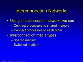
INs in Supercomputers PE PE PE PE PE Mem Mem Mem Mem Mem PE PE PE PE PE Network Network Memory Memory Memory Distributed memory Model Of Supercomputers Dance-Hall Model Of Supercomputers
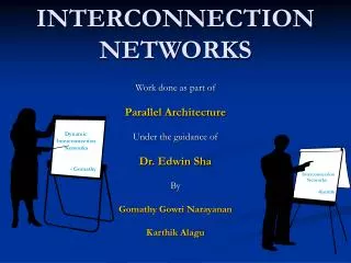
INs in Routers Network Output Line card Input Line card Output Line card Input Line card Output Line card Input Line card Output Line card Input Line card Output Line card Input Line card Output Line card Input Line card Control Processor
Generations of Interconnection Networks 10 Gigabit Ethernet
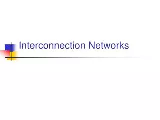
Example Intercon. Networks Mesh Network Communication Links Processing Element (CPU + Mem + other)
Example Intercon. Networks Torus Network Communication Links Wrap around Connections Processing Element (CPU + Mem + other)
Example Intercon. Networks Tree Network Control Element Communication Links Processing Element (CPU + Mem + other)
Crossbar Network • Simplest and most flexible switch architecture • Can establish n connections between n inputs and n outputs • Each X-point can be switched on/off by controller • Number n is often called the degree of the switch `
Classes of Interconnection Nets • Connectivity and control can be used to divide INs into two classes: static and dynamic • Static networks – that don’t change dynamically (e.g., trees, rings, meshes (not crossbars)) • Dynamic networks – that change interconnectivity dynamically – use switched channels
Static Networks • Topological properties particularly important for static networks • Node degree: number of edges incident on a node • Network diameter: diameter D of a network is the maximum path length between any two nodes -- the path length is measured in terms of links traversed
Dynamic Networks • Dynamic networks can be split into • Shared media designs • Switched media designs • Cost increases when converting from shared media to switched design Switched Links Design Shared Media Design
Switched Networks • Switched networks can be: circuit switching or packet (cell) switching • Circuit switched networks -- the entire path from the source to the destination is reserved for the entire period of transmission • Packet switched networks – message is transmitted in packets. Packets are routed in stages.
Packet Switching • Cell switching – is a variation of packet switching where packet size is fixed. • A cell contains a header (routing information – e.g., a label) and payload • Cells from the same message or source can be routed along different paths
Switching Schemes • Two ways of sending packets in switched networks: • Store-and-forward • Cut-through or wormhole routing Store-and-Forward • Entire packet is stored in a node before it is forwarded to an outgoing link • Successive packets are transmitted sequentially without overlapping in time
Switching Schemes Cut-through Routing • Each node uses a flit-buffer to hold a flit (one cell) • A flit is automatically forwarded to an outgoing link, once the header is decoded • All data flits in the same packet follow the same path that the header traverses
Switching Schemes • Using the cut-through it takes only 7 time units for node 4 to receive the entire message • The same message took 16 time units in the store-and-forward scheme
Network Performance Metrics • Communication latency • software overhead: overhead associated with sending and receiving messages at end stations • channel delay: caused by the channel occupancy • routing delay: time spent in the successive switches in making a sequence of routing decisions along the routing path • contention delay: caused by traffic contentions in the network
Network Performance Metrics • Per-port bandwidth: maximum number of bits that can be transmitted per second from any port to any other port • For symmetric network, per-port bandwidth is independent of port location • For asymmetric network, depends on port location • Aggregate bandwidth: defined as the maximum number of bits that can be transmitted from one half of the nodes to another half of the nodes per second
Network Performance Metrics • For example, for 512-port HPS with 40MB/s per-port bandwidth, the aggregate bandwidth = (40x512)/2 = 10.24GB/s
Routing on Static Networks Meshes and Rings: • Simplest connection topology is the one-dimensional mesh, or linear array • In a linear array, the interior nodes have two connections and boundary nodes have one • If we connect the two boundaries, we get a ring with all nodes of degree 2 • A higher dimensional mesh is constructed similarly with k dimensions, interior nodes have degree 2k
Routing on Static Networks… • Common mesh topology is the 2-D mesh • Some 2-D meshes have wrap-around connections along the edges Routing: • Assume interior nodes – routing performed over one dimension at a time • On a 3-D mesh, minimal path from a node (a, b, c) to (x, y, z) is constructed by moving along 1st dimension to (x, b, c) then to (x, y, c) and finally to (x, y, z) • This is known as the XY-routing
Routing on Static Networks … Trees: • Common tree topology is the binary-tree • Binary trees are well matched for VLSI and other planar layouts
Routing on Static Networks… Routing in trees • Idea: travel up the tree from A until you reach an ancestor of B and then travel down • To implement number the root as 1 and left and right children as of x as 2x and 2x+1, respectively • If the root is at level 1 • Then the nodes at level i have a label that is i bits long and the left and right children of a node have 0 or 1 appended to their parent’s number, respectively
Routing on Static Networks… • Lowest common ancestor of A (source) and B (destination) is the node numbered P, the longest common prefix of A and B • From this it is easy to see how many levels we should go up to reach B from A What is this tree called?
Routing in Trees 0001 0010 0011 0100 0101 0111 0110 1111 1010 1011 1100 1101 1110 1000 1001 Src1010 Dst1110 1 (longest common prefix) & 110 remainder on dst Node 0001 is the common ancestor; use 110 to route down from ancestor 110 right, right, left from 0001 (common ancestor)
Routing on Static Network… Hybercubes: • Multidimensional mesh of processors with exactly two processors in each dimension • D-dimensional hypercube has p = 2D • Recursively constructed as follows: • a single processor is 0-dim hypercube • 1-dim hypercube is constructed by connecting two 0-dim hypercubes • (d+1)-dim hypercube is constructed by connecting corresponding processors of two d-dim hypercubes
Routing on Static Network… • Properties of hypercube network • two processors are connected by a direct link if and only if the binary representation of their labels differ at exactly one bit position • in a d-dimensional hypercube, each processor is directly connected to d other processors • a d-dimensional hypercube can be partitioned into two (d-1)-dimensional sub-hypercubes • total number of bit positions at which these two labels differ is called the hamming distance
Routing on Static Network… Routing: E-Cube routing • Let s and d be the labels of the source and destination nodes respectively • Minimum distance between the processors is given by x = (s XOR d) • Processor s sends the message along dim k, where k is the position of the least significant non-zero bit in (s XOR d)
Routing on Static Network… • Processor i computes (i XOR d) and forwards the message along the dimension corresponding to the least significant nonzero bit
Dynamic Network Topologies • Examples: • Buses, Crossbars, and Multistage interconnection networks • Supercomputers, high performance IP routers, ATM switches use these networks (e.g., IBM DeepBlue) • Several aliases - omega, flip, butterfly, baseline, delta, generalized cube, multistage shuffle-exchange
Multistage Cube Network • Cross-bar has several advantages • Allows different types of connection patterns – unicast, broadcast, multicast • Has n2 switch cost – not very scalable • Multistages switches – build cheaper and scalable switches that can provide “large” number of connection patterns • Reduce switch cost (n2 n log n)
Multistage Cube Network Cross Bar Switch Cross Bar Switch Cross Bar Switch Cross Bar Switch Cross Bar Switch Cross Bar Switch Cross Bar Switch Cross Bar Switch Cross Bar Switch Cross Bar Switch
Multistage Cube Network • For a NxN network, we have m = log2N stages • Each stage has N/2 two-input/two-output interchange boxes • The connection pattern among the boxes is different for the different multistage interconnection networks (MINs) P P cubei(P) cubei(P)
Multistage Cube Network • cubei(P) is the cube interconnection function • Let P = pm-1...pi...p1p0 • cubei(P) = pm-1...pi...p1p0 • Each box can be controlled by routing tags -- in one of the following four states
Multistage Cube Network Routing in multistage cube networks: • Circuit-switching – all switches in a stage set the same way • Packet switching – each packet has routing tag in its header and the routing can be performed in a distributed fashion • Less overhead for circuit switching – almost like a direct wire connection
Multistage Cube Network • Unicast routing: routing between a sender and a receiver • XOR routing tags • Let source be S and destination be D • tag T = S XOR D • If circuit switching is used, stage i is set straight if bit i of T is 0 otherwise stage i is set exchange • If packet switching is used, each box is set independently by the header (tag is sent in the header) of the packet
Multistage Cube Network Destination Routing Tag • Let S be the source and D be the destination • Tag = D • This is used in distributed fashion -- each network input device determines its own action • Tag is sent in the header for the message • Stage i box examines di • di = 0 use upper box output • di = 1 use lower box output
Multistage Cube Network • Trade-offs between the two routing schemes for MINs • XOR tag can be used for return message and source information • T = S XOR D = D XOR S; S = D XOR T • destination tag can be used to check the correct destination
Multistage Cube Network Broadcast routing: • One port to 2j ports -- note this is a restriction -- this is not a multicast where you can have an arbitrary set of receivers • The receivers can have at most j bits different between any pair of destination addresses • port S -> ports { D1, D2, ... D2j} • unicast routing tag R = S XOR D1 • broadcast tag B = Di XOR Dk (must differ in at least j positions)
Multistage Cube Network • Stage i looks at the i-th bit of routing tag R (ri) and broadcast tag B (bi) • If bi = 0, use ri 1 exchange, 0 straight • If bi = 1, broadcast (ignore ri)
Multistage Cube Network Example • Source S = 2 = 010 • Destinations = {100, 101, 110, 111} • Vary at most 2 bits • R = S XOR 100 = 110 • B = 100 XOR 111 = 011