Download
1 / 29
310 likes | 501 Views
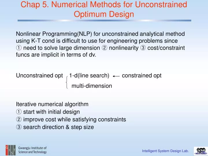
Chap 5. Numerical Methods for Unconstrained Optimum Design. Nonlinear Programming(NLP) for unconstrained analytical method using K-T cond is difficult to use for engineering problems since ① need to solve large dimension ② nonlinearity ③ cost/constraint funcs are implicit in terms of dv.

E N D
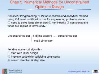
Chap 5. Numerical Methods for Unconstrained Optimum Design Nonlinear Programming(NLP) for unconstrained analytical method using K-T cond is difficult to use for engineering problems since ① need to solve large dimension ② nonlinearity ③ cost/constraint funcs are implicit in terms of dv. Unconstrained opt 1-d(line search) constrained opt multi-dimension Iterative numerical algorithm ① start with initial design ② improve cost while satisfying constraints ③ search direction & step size Intelligent System Design Lab.
Search direction : steepest descent method conjugate gradient method newton’s method quasi-newton method Step size : equal interval search golden section search polynomial interpolation (1-d) Intelligent System Design Lab.
Iterative numerical algorithm Unconstrained : depend on f, Δf Constrained : depend on f, Δf, g, Δg Descent step Intelligent System Design Lab.
Descent cond 90˚~270˚ Rate of convergence : no of iteration no of func evaluation Intelligent System Design Lab.
Numerical Gradient Calculation FD – FFD, BFD, CFD Semi-analytical Analytical – discrete, continuum – DDM, AVM Automatic differentiation (ADIFOR, ADIC : Rice Univ) Step size α Intelligent System Design Lab.
Equal Interval search Improved equal interval Alternate method Discard 1/3 and repeat Intelligent System Design Lab.
δ rδ r2δ r3δ Golden section search (r >1) r=1.618 (golden ratio) Intelligent System Design Lab.
1, 1, 2, 3, 5, 8, 13, 21, 34, 55, Fibonacci sequence τ=0.618, 1-τ=0.382=τ2 Intelligent System Design Lab.
Polynomial Interpolation f(a) : real function q(a) : approximated function a * : real minimum : approximated minimum Intelligent System Design Lab.
Ex. 5.4 Intelligent System Design Lab.
Ex 5.6 One-dimensional minimization with quadratic interpolation Find the minimum point of by polynomial interpolation. Use Golden Section search δ=0.5 initially to bracket the minimum point. sol Iteration 1. From Example 5.5 the following information is known. The coefficients a0, a1 and a2 are calculated from Eqs(5.30) as Therefore, =1.2077 from Eqs (5.31), and =0.5149. Note that and . Thus, new limits of the reduced interval of uncertainty are Intelligent System Design Lab.
Iteration 2. We have the new limits for the interval of uncertainty, the intermediate point and the respective values as The coefficients a0, a1 and a2 are calculated as before, a0=2.713, a1=-7.30547, and a2=5.3807. Thus =1.3464 and =0.4579. Comparing with the optimum solution given in Table 5.2, we observe that and are quite close to the final solution. One more iteration can give very good approximation to the optimum. Note that only 5 function evaluations are required to obtain a fairly accurate optimum step size for the function f(α). Therefore, the polynomial interpolation approach can be quite efficient for one-dimensional minimization. Intelligent System Design Lab.
Steepest Descent Method Steepest descent method - first order Gradient method second order Steepest descent method Steepest descent direction Intelligent System Design Lab.
Steepest Descent Method EX. minimize using steepest descent method Intelligent System Design Lab.
Steepest Descent Method Intelligent System Design Lab.
Steepest Descent Method Pro : simple, robust, convergent Con : slow convergence (many iteration req’d) due to first order inefficient since compute every iteration direction of steepest descent is good only locally rate of convergence is linear Cond(A)=λ1/ λn ≥0 λ12 : largest eigenvalue of ATA, λn2 : smallest Large cond number means A is nearly singular. Intelligent System Design Lab.
Ex. 5.10 Use of steepest descent algorithm Minimize using the steepest descent method with a starting design as (2, 4, 10). Select the convergence parameter ε as 0.005. Perform a line search by Golden Section search with initial step length δ=0.05 and an accuracy of 0.0001. sol Intelligent System Design Lab.
Note that which verifies the line search termination criterion. The steps in steepest descent algorithm should be repeated until the convergence criterion is satisfied. Appendix D contains the computer program and user supplied subroutines FUNCT and GRAD to implement steps of the steepest descent algorithm. The iterative history for the problem with the program is given in Table 5.3. The optimum cost function value is 0.0 and the optimum point is (0, 0, 0). Note that a large number of iterations and function evaluations are needed to reach the optimum Intelligent System Design Lab.
Scaling of DV to improve convergence If cond(H)=1, SDM converges in one iteration For , calculate H, and let Where are eigenvector of H and are eigenvalues Then converges in one iteration, Intelligent System Design Lab.
Conjugate Gradient Method Intelligent System Design Lab.
Example 5.13 Use of conjugate gradient algorithm. Solution. The first iteration of the conjugate gradient The second iteration Intelligent System Design Lab.
Example The design is updated as Computing the step size to minimize , we get Substituting this into the above expression, we get Calculating the gradient at this point we get , so we need to continue the iteration. Note that Intelligent System Design Lab.
Newton’s Method Use second-order info(Hessian) thus quadratic convergence does not guarantee to converge Modified Newton’s Method Marquardt Modification When is large, H is neglected, steepest descent When is small, Newton method Far away from soln, SDM : near optimum, Newton method Intelligent System Design Lab.
Quasi-Newton Method(1) Use first-order info to approximate Hessian Use results of previous iteration DFP(Davidon-Fletcher-Powell Method) Intelligent System Design Lab.
Quasi-Newton Method(2) BFGS(Broyden-Fletcher-Goldfarb-Shanno) method Intelligent System Design Lab.
Transformation methods for Optimum Design Constrained OD Unconstrained OD transform penalty multiplier P : penalty func r : control parameter Sequential Unconstrained Minimization Techniques(SUMT) penalty function barrier function (for inequality) Disadvantages : penalty and barrier funcs ill-behave near the boundary of function region Intelligent System Design Lab.
Multiplier (Augmented Lagrangian) Methods – LM+Penalty Improve SUMT - good conditioning - convergent - fast convergence Intelligent System Design Lab.