Download
1 / 42
540 likes | 1.14k Views
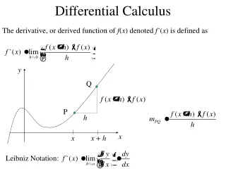
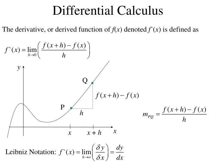
Differential Calculus. The derivative, or derived function of f ( x ) denoted f` ( x ) is defined as . y. Q. P. h. x. x. x + h. Given that f(x) is differentiable, we can use the definition to prove that if . Differentiation from first principles.

E N D
Differential Calculus The derivative, or derived function of f(x) denoted f`(x) is defined as y Q P h x x x + h
Given that f(x) is differentiable, we can use the definition to prove that if Differentiation from first principles
Further practice on page 29 Exercise 1A Questions 1, 4, 5 and 7 TJ Exercise 1 But not just Yet……..
y x Not all functions are differentiable. CAUTION y = tan(x). Here, tan(x) has ‘breaks’ in the graph where the gradient is undefined Although the graph is continuous, the derivative at zero is undefined as the left derivative is negative and the right derivative is positive. For a function to be differentiable, it must be continuous.
Further practice on page 29 Exercise 1A Questions 1, 4, 5 and 7 TJ Exercise 1 Differentiation reminder: Page 32 Exercise 3A Questions 1(a), (d), 2(a), (c), (d) 3(a), 4(a), 6(a) TJ Exercise 2 TJ Exercise 3
The Product Rule Using Leibniz notation, OR
Page 35 exercise 4A Questions 1, 2(b) and 3 Page 36 exercise 4B Questions 1(b), 3 and 4 TJ Exercise 4
The Quotient Rule Using Leibniz notation, OR
Page 37 exercise 5A Questions 1 to 4 and 7 Page 38 Exercise 5B Questions 1 to 3 TJ Exercise 5
Sec, Cosec, cot and tan Unlike the sine and cosine functions, the graphs of sec and cosec functions have ‘breaks’ in them. The functions are otherwise continuous but for certain values of x, are undefined.
(quotient rule) Page 40 Exercise 7 questions 1, 2, 3(a), (c), (e), (g). 4(a) TJ Exercise 6 Questions 1 to 4
Proof 1. Let us examine this limit. When a approaches e, the limit approaches 1.
Proof 2. Differentiating both sides with respect to x. Using the chain rule.
Higher derivatives Function 1st derivative 2nd Derivative………..nth Derivative etc. etc. etc.
Page 43 Exercise 8A Questions 1(b), (d), 2(b), (c), (d), 3(a), (b),(c). 4(d), (e), 5(a), (c), (e), 6(b), (c),(e) TJ Exercise 6 Page 46 Exercise 9A Qu. 1 to 6 Review Chapter 2.1
Applications of Differential Calculus Let displacement from an origin be a function of time. Velocity is a rate of change of displacement. Acceleration is a rate of change of velocity. Note: The use of units MUST be consistent.
A particle travels along the x axis such that • x(t) = 4t3 – 2t + 5, • where x represents its displacement in metres from the origin ‘t’ seconds after observation began. • How far from the origin is the particle at the start of observation? • Calculate the velocity and acceleration of the particle after 3 seconds. Hence the particle is 5m from the origin at the start of the observation.
A body travels along a straight line such that • S = t3 – 6t2 + 9t + 1, • where S represents its displacement in metres from the origin after observation began. • Find when (i) the velocity and (ii) the acceleration is zero. • When is the distance S increasing? • When is the velocity of the body decreasing? • Describe the motion of the particle during the first 4 seconds of observation.
The velocity is zero when t = 1 or 3 seconds. The acceleration is zero when t = 2 seconds.
This occurs when the graph of is above the x axis (b) S is increasing when Hence the distance S is increasing when t < 1 and when t > 3 seconds. (c) V is decreasing when Hence the velocity is decreasing when t < 2 seconds.
At t = 0, the particle is 1m from the origin with a velocity of 9ms-1 decelerating at a rate of 12ms-2. At t = 1, the particle is 5m from the origin at rest decelerating at a rate of 6ms-2. At t = 2, the particle is 3m from the origin with a velocity of -3ms-1 with zero acceleration. At t = 3, the particle is 1m from the origin at rest accelerating at a rate of 3ms-2. At t = 4, the particle is 5m from the origin with a velocity of 9ms-1 accelerating at a rate of 12ms-2.
Page 51 Exercise 1 Questions 1(a), (b), (d), (f), 2(a), (c), (e), 3, 4, 6, 7, 8, 10, 12. TJ Exercise 7.
Extreme Values of a Function(Extrema) Critical Points A critical point of a function is any point (a, f(a)) where f `(a) = 0 or where f `(a) does not exist.
Critical points are: A (-2,4) f `(-2) does not exist. (Right differentiable at x = -2) A E B (0,0) f `(0) = 0. (Turning point) D C C (1,1) f `(1) does not exist. Left derivative =2, right derivative = 1 B D (2,2) f `(2) does not exist. Left derivative = 1, right derivative = 0.5 E is not a critical point as it is not in the domain of f.
Local extrema Local extreme values occur either at the end points of the function, turning points or critical points within the interval of the domain. Consider the function, 3 is the local maximum value -1 is the local minimum value If extrema occurs at end points then they are end point maximums or end point minimums.
In short, • Local maximum / minimum turning points • End point values • Critical points The Nature of Stationary Points. If f `(a) = 0 then a table of values over a suitable interval centred at a provides evidence of the nature of the stationary point that must exist at a. A simpler test does exist. It is the second derivative test.
If the second derivative test is easier to determine than making a table of signs then this provides an efficient technique to finding the nature of stationary points. Page 56 Exercise 2 Questions 1, 3(a), (c), (e), (g), (i) Page 60 Exercise 3 Questions 1(a), (c), (e), 5(a) to (d) TJ Exercise 8
Optimisation Problems Optimisation problems appear in many guises – often in the context in which they are set can be somewhat misleading. • Read the question at least TWICE. • Draw a sketch where appropriate. This should help you introduce any variables you are likely to need. It may be that you come back to the diagram to add in an extra ‘x’ etc. • Try to translate any information in the question into a mathematical statement. • Identify the variables to be optimised and then express this variable as a function of one of the other variables. • Find the critical numbers for the function arrived at in step 4. • Determine the local extrema and if necessary the global extrema.
(max / min V occurs when = 0) 1. An open box with a rectangular base is to be constructed from a rectangular piece of card measuring 16cm by 10cm. A square is to be cut out from each corner and the sides folded up. Find the size of the cut out squares so that the resulting box has the largest possible volume. x 16 – 2x x 10 – 2x
Page 63 Exercise 4A. Note Question 8 can’t be done but try to prove me wrong!! Page 64 Exercise 4B is VERY Difficult. (VERY) TJ Exercise 9