Download
1 / 17
210 likes | 262 Views
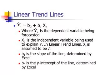
Forecasting Models With Linear Trend. Linear Trend Model. y-intercept. Random Error at Period t. Slope. Value of the time series at Period t. If a time series is hypothesized that has only linear trend and random effects, it will be of the form:

E N D
Forecasting Models With Linear Trend
Linear Trend Model y-intercept Random Error at Period t Slope Value of the time series at Period t • If a time series is hypothesized that has only linear trend and random effects, it will be of the form: • To check if this model is appropriate run a regression analysis and check to see if you can conclude that β1 ≠ 0. • Conclude β1 ≠ 0 if there is a low p-value for this test. yt = β0 + β1t + εt
Forecasting Methods For Models With Long Term Trend • Regression • Places equal weight on all observations in determining a “best straight line”. • Holt’s approach • Rather than calculate one straight line, this approach uses exponential smoothing twice (once to update the smoothed “level” and once to update the estimate for the slope. • It places more weight on the more recent time series values.
Regression Forecasting MethodBasic Approach • Construct the regression equation based on the historical data available for n periods using • Y (dependent variable) -- time series values • X (independent variable) – period values (1, 2, etc.) • Extend the regression line into the future to generate future forecasts • Since regression is only technically valid within the observed values of the independent variable (periods 1 through n) the forecast should not be extrapolated too far into the future (beyond period n).
Regression Forecasts • Regression will return the best straight line that fits through the set of time series values: b0 + b1t. Forecast for Period k Fk = b0 + b1k
Example • Standard and Poor’s (S&P) is a bond rating firm and is conducting an analysis of American Family Products Corp. (AFP). • They need to forecast of year-end current assets for years 11, 12 and 13, based on time series data for the previous 10 years given below in $millions.
Plot the Time Series Long term linear trend does appear to be present Verify using regression!
Regression Output L0W p-value Can conclude LINEAR TREND
Forecasts for Periods 1 -13 =$I$17+$I$18*A2 Drag C2 down to cells C3:C14 Forecasts for Years 11,12 and 13 • Enter 11, 12 and 13 in cells A12, A13 and A14
Performance Measures for Regression Approach =ABS(D2)/B2 =ABS(D2) =B2-C2 =D2^2 =AVERAGE(E3:E11) =AVERAGE(F3:F11) =AVERAGE(G3:G11) =MAX(F3:F11) Drag D2:G2 to D11:G11
Holt’s ApproachBasic Concepts • Smooths current point to a point Lt • Re-evaluates the trend from one period to the next based on the new time series value, Tt • Forecast for the next period, t+1, starts from the smoothed level Lt and changes by Tt(1) since the next period is one period into the future: Ft+1 = Lt + Tt • The forecast for k periods from period t is: Ft+k = Lt + Tt(k) • Forecast changes when additional time series data is observed.
Initial Values for Holt’s Approach • Need some initial values for L2 and T2 • Conventional starting values: • Since this is a “trend” model, 2 points are needed to get started • The initial “smoothed” trend at time 2 is just the observed trend that did occur between periods 1 and 2: • The initial level, the level at period 2 is set to the actual time series value at period 2: • First forecast is for period 3: • T2 = y2 - y1 • L2 = y2 • F3 = L2 + T2
Holt’s Approach Exponential smoothing is then done to determine: Ft+1 = Lt + Tt Lt= Level = exponentially smoothed value for current period Tt = Trend = exponentially smoothed value for the slope for current period A representative value of where the time series “should be” at time t A representative value of what the slope “should be” at time t Exponential smoothing based on: Actual value at time t -- yt Forecasted value for time t -- Ft Exponential smoothing based on: Difference in last two levels Lt - Lt-1 Forecasted value for time t-1 – Tt-1 Lt = yt+ (1- )Ft Tt = (Lt-Lt-1)+ (1- )Tt-1 Forecast for next period, t+1: Ft+1 = Lt + Tt
Excel: Holt’s ApproachInitialization =B3 =B3-B2 =C3+D3
Excel: Holt’s ApproachRecursive Calculations =.1*B4+.9*E4 =.2*(C4-C3)+.8*D3 Drag C4:E4down to C11:E11 • Smoothing constant for the level: α = .1 • Smoothing constant for the trend: = .2
Excel Holt’s ApproachForecasts =C11+D11 =E12+$D$11 Absoluteaddress of last trend estimate Relativeaddressof last forecast Drag E13 down to E14
Review • Scatterplot to observe trend • Regression to verify linear trend • Low p-value for t-test for 1 • Models with Trend and Random Effects Only • Linear Regression • Holt’s Technique • Use of Performance Measures to do comparisons