Download
1 / 34
350 likes | 505 Views
Search Problems. CSD 15-780: Graduate Artificial Intelligence Instructors: Zico Kolter and Zack Rubinstein TA: Vittorio Perera. Search. Search lectures. Readings: Section II in Norvig and Russel (chapters 3,4, 5, and 6). Today ’ s lecture.

E N D
Search Problems CSD 15-780: Graduate Artificial Intelligence Instructors: ZicoKolter and Zack Rubinstein TA: Vittorio Perera
Search • Search lectures. • Readings: • Section II in Norvig and Russel (chapters 3,4, 5, and 6)
Today’s lecture • Why is search the key problem-solving technique in AI? • Formulating and solving search problems. • Understanding and comparing several “blind” or uniformed search techniques.
Projects Multi-robot movement planner for robust, just-in-time delivery of components for wing ladder assembly (Boeing) MARTI – Market-based dynamic allocation of tasks to RF devices to perform secondary mission requests (DARPA RadioMap) Assessment Region REVAMP - Same-day scheduler and real-time itinerary execution management support for paratransit operations. (ongoing ACCESS pilot) • SURTRAC - Adaptive traffic signalization control system • Focus on evaluation • (pilot and expansion) SMOS - Cross-operations (air, cyber, space) coarse-level planner for missions (BAE and AFRL)
Examples of “toy” problems • Puzzles such as the 8-puzzle: • Cryptarithmetic problems: SEND 9567 MORE+1085 MONEY 10652
The n-queens problem • A popular benchmark for AI search • Solved for n up to 500,000
Explicit solution for n ≥ 4 [Hoffman, Loessi, and Moore, 1969] If n is even but not of the form 6k+2: For j = 1, 2, ..., n/2 place queens on elements (j, 2j), (n/2+j, 2j-1) If n is even but not of the form 6k: For j = 1, 2, ..., n/2 place queens on elements (j, 1+[(2(j-1) + n/2 - 1) mod n]), (n+1-j, n-[(2(j-1) + n/2 - 1) mod n]) If n is odd: Use case A or B on n-1 and extend with a queen at (n,n) Is this a good benchmark problem for testing search techniques?
Real-world problems • Signal interpretation (e.g. speech understanding) • Theorem proving (e.g. resolution techniques) • Combinatorial optimization (e.g. VLSI layout) • Robot navigation (e.g. path planning) • Factory scheduling (e.g. flexible manufacturing) • Symbolic computation (e.g. symbolic integration) Can we find closed form solutions to these problems?
Formulating search problems • States and state spaces • Operators - representing possible actions • Successor function • Initial state and goal test • Path cost function Examples: 8-puzzle, 8-queen, path planning, map coloring. What are the corresponding states, operators, initial state, goal test, and path cost.
States, Operators, Successor function. State – choose data representation, e.g., 3x3 2D array with numbers and 0 representing the blank. move-left, move-right, move-up, move-down. Operators – transform state to next state, e.g., possible movements for the blank. Successor Function – generate possible states by applying operators, e.g., apply operators and return states whose indices are between 1 and 3.
What is a solution? • A solution to a search problem is a sequence of operators that generate a path from the initial state to a goal state. • An optimal solution is a minimal cost solution. • Solution cost versus search cost.
Choosing states and actions • Efficiency versus expressiveness • The use of abstraction: • Ignore road condition travel planning. • Use job description and ignore names in task scheduling. • Ignore the color of the pieces when solving the 8-puzzle. • Compact action representation.
Quote for the day “The problem of searching a graph has effectively been solved, and is no longer of interest to AI researchers.” - Nils Nilsson, early 1970s
Searching for solutions Search control strategies • Order in which the search space is explored • The extent to which partial solutions are kept and used to guide the search process • The degree to which the search process is guided by domain knowledge • The degree to which control decisions are made dynamically at run-time
Evaluation of search strategies • Completeness - does it guarantee to find a solution when there is one? • Time complexity - how long does it take to find a solution? • Space complexity - how much memory does it require? • Optimality - does it return the best solution when there are many?
Search trees • A graph representing the search process • Implicit graphs and explicit graphs • Branching factor and depth • Generating and expanding states • Open and closed lists of nodes • Representing a node of the explicit graph: class Node: State = None ParentNode = None Operator = None Depth = None PathCost = None
Blind search strategies • Depth-first search • Breadth-first search • Depth-limited search • Iterative-deepening search • Bidirectional search
Depth-First Search functiondfs (nodes, goalp, successors) returns solution or fail if not nodes thenreturn fail elseifgoalp(first(nodes)) thenreturn first(nodes) elsereturndfs(append(successors(first(nodes)), rest(nodes)), goalp, successors)
Example Road Network A 10 12 B C 8 4 4 F E D 8 4 6 H G 20 6 12 I DFS(AI): A, B, D, G, I = 36
Time and Space Complexity of DFS • Let b be the branching factor and m be the maximum depth of the state space. • Space complexity = bm • Time complexity = O(bm) • Complete? • Optimal?
Breadth-First Search functionbfs (nodes, goalp, successors) returns solution or fail if not nodes thenreturn fail elseifgoalp(first(nodes)) thenreturn first(nodes) elsereturndfs(append(rest(nodes), successors(first(nodes))), goalp, successors)
Example Road Network A 10 12 B C 8 4 4 F E D 8 4 6 H G 20 6 12 I BFS(AI): A, C, F, I = 36
Time and Space Complexity of BFS • Let b be the branching factor and d be the depth at which a solution is found. • Space complexity = O(bd) • Time complexity = O(bd) • Complete? • Optimal?
Uniform-Cost Search functionucs (nodes, goalp, successors) returns solution or fail nodes = sort(<, nodes, node.cost) if not nodes thenreturn fail elseifgoalp(first(nodes)) thenreturn first(nodes) elsereturnucs(append(rest(nodes), successors(first(nodes))), goalp, successors) • Time and space complexity?
Example Road Network A 10 12 B C 8 4 4 F E D 8 4 6 H G 20 6 12 I UCS(AI): A, C, E, H, I = 26
Uniform Cost Search Properties • Guaranteed to find lowest cost solution (optimal and complete) as long as cost never decreases. • Same complexity as Breadth-First search • Space complexity = O(bd) • Time complexity = O(bd)
Depth-Limited Search • Same as DFS, except depth threshold used to limit search. • Similar time and space complexity to DFS, except bounded by threshold. • Be careful to choose an appropriate threshold • Complete? • Optimal?
Example Road Network A 10 12 B C 8 4 4 F E D 8 4 6 H G 20 6 12 I DLS(AI,4): A, B, D, G, I = 36
Iterative Deepening Search • Do repeated Depth-Limited searches, while incrementally increasing the threshold. • Similar time and space complexity to DFS, except bounded by depth of the solution. • Does redundant expansions. • Is complete and optimal.
Example Road Network A 10 12 B C 8 4 4 F E D 8 4 6 H G 20 6 12 I IDS(AI): A, C, F, I = 36
Bidirectional search • Time and space complexity: bd/2 When is bidirectional search applicable?
Time and Space Complexity of Bidirectional Search • Time Complexity = O(bd/2) • Space Complexity = O(bd/2) • High space complexity because the nodes have to be kept in memory to test for intersection of the two frontiers.