Download
1 / 66
670 likes | 785 Views
Demand. Indifference Mapping - A Bottom-up Approach. Important Economic Concepts. Utility Scarcity Sacrifice and Opportunity Cost Ceteris paribus Law of Diminishing Marginal Utility. Indifference Analysis. Consumer Choice.

E N D
Demand • Indifference Mapping - A Bottom-up Approach
Important Economic Concepts • Utility • Scarcity • Sacrifice and Opportunity Cost • Ceteris paribus • Law of Diminishing Marginal Utility
Indifference Analysis Consumer Choice • Since it is difficult to directly measure utility, a technique called indifference analysis is used which measures utility indirectly by observing how a consumer behaves when faced with choices between two goods.
Indifference Analysis Consumer Choice • Would you prefer six donuts and three bananas or five donuts and four bananas? • The consumers behavior with respect to two commodities is best viewed graphically.
A Consumers Choice • When faced with choosing between two combinations of two goods (i.E. Six donuts and three bananas or five donuts and four bananas) there can only be one of three responses; You prefer six donuts and three bananas over five donuts and four bananas, You prefer five donuts and four bananas over six donuts and three bananas, or You are just as happy with either combination; You are indifferent
Dealing With Complexity • The economic world is a complex and dynamic environment. • Everything is connected to a greater or lesser degree.
Ceteris Paribus Everything Else Held Constant In order to study specific parts of the economy, it is necessary to simplify the situation by choosing two or three things to observe and “freezing” everything else.
Ceteris Paribus Everything Else Held Constant If we want to study an individuals demand for donuts at various prices, we must assume that everything else is held constant, i.E. Price of bananas, the consumers income, etc.
Indifference Mapping An example • A student, Susan, is given a weekly allowance to spend on lunch. She spends her money on milkshakes and hamburgers. • What are her choices?
Susan’s Indifference Curve • There will be several different combinations of burgers and shakes which will yield the same level of utility to Susan. • A line connecting these combinations is called an indifference curve.
MARGINAL RATE of SUBSTITUTION (MRS) • MRS = the rate at which the consumer will exchange one good for the other. • MRS = the ratio of the marginal utility of good A to the marginal utility of good B. • MRS = the slope of the indifference curve.
Indifference Map Just Like a Topography Map • The graph is a solid surface of possible indifference curves. • When several curves are shown, this is referred to as an “indifference map.”
Susan’s Budget We All Have to Live Within a Budget • Susan, is given a weekly allowance of $7.50 to spend on lunch. • Milkshakes and hamburgers cost $0.50 and $1.00 respectively.
Consumer Behavior Assuming Susan Spends All of Her Allowance • Susan will eventually find the number of burgers & shakes she can afford each week that suits her best. • A consumer will always move up and down the budget line seeking the combination which yields the highest utility. • At that point the MRS will equal the price ratio.
Optimum combination (3.5*$1 + 8*$0.50) = $7.50
Consumer Equilibrium At the Optimum Combination on the Budget Line • MUm/MUh = Pm/Ph, or • MUm/Pm = Muh/Ph, or • Where MRS = Pm/Ph
The Effect of Price Changes On Consumer Equilibrium • If the price of milkshakes drops from 50 cents to 30 cents, the budget line will pivot out, all indifference curves are unchanged. • But there is a new point where the MRS equals the new price ratio.
New Consumer Equilibrium • Since the graph is a solid surface of budget lines, there will be one that just touches the new budget line. • At the new price there will be a new, higher budget line and consumer equilibrium point. • At the new tangency, more shakes and more or fewer burgers will be purchased.
Finding Susan’s Demand for Milkshakes • We now have enough information to construct Susan's demand curve. • A demand schedule is defined as a list of prices and the quantities at each price that a consumer will be willing and able to purchase.
Q 1.50 12 1.25 10 1.00 8 .75 6 .50 4 .25 2 2 2 4 4 6 6 8 8 10 10 12 12 14 14 16 16 TB/Pb TB = Total budget Pb = Price of burgers Pm = price of milkshakes Hamburgers TB/Pm Quantity Milkshakes Price of milkshakes Quantity Milkshakes
Q 1.50 12 1.25 10 1.00 8 .75 6 .50 4 .25 2 2 2 4 4 6 6 8 8 10 10 12 12 14 14 16 16 TB/Pb TB = Total budget Pb = Price of burgers Pm = price of milkshakes Hamburgers TB/Pm Where Pm= 1.25 Quantity Milkshakes Price of milkshakes Quantity Milkshakes
Q 1.50 12 1.25 10 1.00 8 .75 6 .50 4 .25 2 2 2 4 4 6 6 8 8 10 10 12 12 14 14 16 16 TB/Pb TB = Total budget Pb = Price of burgers Pm = price of milkshakes Hamburgers TB/Pm Where Pm= 1.00 The price of shakes decreases Which results in an increase in consumption Quantity Milkshakes Price of milkshakes Quantity Milkshakes
Q 1.50 12 1.25 10 1.00 8 .75 6 .50 4 .25 2 2 2 4 4 6 6 8 8 10 10 12 12 14 14 16 16 TB/Pb TB = Total budget Pb = Price of burgers Pm = price of milkshakes Hamburgers TB/Pm Quantity Milkshakes Where Pm= .75 The price of shakes decreases further Which results in another increase in consumption Price of milkshakes Quantity Milkshakes
Q 1.50 12 1.25 10 1.00 8 .75 6 .50 4 .25 2 2 2 4 4 6 6 8 8 10 10 12 12 14 14 16 16 TB = Total budget Pb = Price of burgers Pm = price of milkshakes Hamburgers Quantity Milkshakes Now we have identified three price-quantity coordinates and can construct Susan’s demand curve Price of milkshakes Quantity Milkshakes
Market Demand • Now that we have found Susan’s demand for milkshakes we can see how aggregate (total market) demand can be found. • Market demand (aggregate demand) is simply the horizontal summation of each individual’s demand curve. • This can be illustrated simply if we assume there are only two individuals in the market; Susan and Joe.
Price per milkshake Price per milkshake Price per milkshake D Ds .75 .75 .75 .50 .50 Dj .50 .25 .25 .25 D Ds Dj Q Q Q 5 10 15 10 20 30 5 10 15
Market Demand (Aggregate Demand) • Just as indifference analysis is bottom-up approach to the study of demand, aggregate demand analysis is a top-down approach to the same subject. • Aggregate demand is the total market demand for a good or service and the concept can have a wide range of applications; • You could look at the world demand for wheat, or. • You could study the demand for hamburgers in the city of Stephenville Texas.
Market Demand (Aggregate Demand) It all depends on how you define the market.
Law of Demand • As price increases the quantity demanded decreases, • As price decreases the quantity demanded increases. • In other words, price and quantity demanded are inversely related.
Demand Curve A list of prices and the quantities of the commodity, at each price, that consumers are willing and able to purchase.
Factors of Demand Things that Affect Demand • Price • Population • Consumer tastes & preferences • Income • Price of substitutes • Price of complements • Seasonality
Graphing a Demand Curve • A graph of demand shows the relationship between two things; -- Price, and. -- Quantity demanded. • A change from one price to another price will result in moving from one point to another along the demand curve, ceteris paribus. • An decrease in price will result in a increase in the quantity demanded.
Changes Other Than Price Relaxing the Ceteris Paribus Assumption • A change in any factor of demand, other than price, will cause there to be a shift in the entire demand curve. • An increase in population will shift demand out (increase demand). • An increase in the price of complements will shift demand in (decrease demand). • In increase in income could cause demand to shift in either direction depending on the com.
Demand Shifters • Population • Consumer tastes & preferences • Income • Price of substitutes • Price of complements
Price Elasticity of Demand Another Important Attribute of Demand • Price Elasticity of Demand some times referred to as Own price elasticity or simply Price Elasticity. • Ep = (% change in Quantity)/(% change in Price) -- Ep < 1 = Inelastic -- Ep > 1 = Elastic -- Ep = 1 = Unitary
Why Price Elasticity Is Important What you should know about the commodities you sell • If Ep is unitary then an increase or decrease in price changes total revenue proportionately • If Ep is inelastic then an increase in price increases total revenue
Why Price Elasticity Is Important What you should know about the commodities you sell • If Ep is inelastic then an decrease in price decreases total revenue • If Ep is elastic then an increase in price decreases total revenue • If Ep is elastic then an decrease in price increases total revenue