Download
1 / 5
50 likes | 138 Views
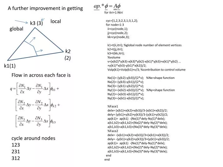
A further improvement in getting. for itri=1:Ntri cyc=[1,2,3;2,3,1;3,1,2]; for node=1:3 ii=cyc(node,1); jj=cyc(node,2); kk=cyc(node,3); k1=t(ii,itri); %global node number of element vertices k2=t(jj,itri); k3=t(kk,itri); %volume

E N D
A further improvement in getting for itri=1:Ntri cyc=[1,2,3;2,3,1;3,1,2]; for node=1:3 ii=cyc(node,1); jj=cyc(node,2); kk=cyc(node,3); k1=t(ii,itri); %global node number of element vertices k2=t(jj,itri); k3=t(kk,itri); %volume v=(x(k2)*y(k3)-x(k3)*y(k2)-x(k1)*y(k3)+x(k1)*y(k2) ... +y(k1)*x(k3)-y(k1)*x(k2))/2; Volp(k1)=Volp(k1)+v/3; %contribution to control volume Nx(1)= (y(k2)-y(k3))/(2*v); %Nx=shape function Nx(2)= (y(k3)-y(k1))/(2*v); Nx(3)= (y(k1)-y(k2))/(2*v); Ny(1)=-(x(k2)-x(k3))/(2*v); %Ny=shape function Ny(2)=-(x(k3)-x(k1))/(2*v); Ny(3)=-(x(k1)-x(k2))/(2*v); %Face1 delx= (x(k1)+x(k2)+x(k3))/3-(x(k1)+x(k2))/2; dely= (y(k1)+y(k2)+y(k3))/3-(y(k1)+y(k2))/2; ap(k1)= ap(k1) -(Nx(1)*dely-Ny(1)*delx); a(k1,k2)=a(k1,k2)+(Nx(2)*dely-Ny(2)*delx); a(k1,k3)=a(k1,k3)+(Nx(3)*dely-Ny(3)*delx); %Face2 delx= -(x(k1)+x(k2)+x(k3))/3+(x(k1)+x(k3))/2; dely= -(y(k1)+y(k2)+y(k3))/3+(y(k1)+y(k3))/2; ap(k1)= ap(k1) -(Nx(1)*dely-Ny(1)*delx); a(k1,k2)=a(k1,k2)+(Nx(2)*dely-Ny(2)*delx); a(k1,k3)=a(k1,k3)+(Nx(3)*dely-Ny(3)*delx); end end local k3 (3) global k2 (2) k1(1) Flow in across each face is cycle around nodes 123 231 312
Boundary conditions: extra data structure Section on boundary 1 3 2 7 5 8 1 6 2 4 7 5 8 3 6 4 1 2 3 3 3 3 4 4 e = 3 8 Boundary number 2 8 5 5 9 10 4 7 6 10 4 9 12 7 6 1 11 11 3 1 2
Global node know from edge array k2 Rewrite equation ion the form k1 Coefficient contribution Constant contribution From one boundary segment Note if insulated If fixed value If fixed flux
Boundary code %Set Boundary conditions %User section assummes user knows how many boundarys and index h(1)=0; h(2)=0; h(3)=1e18; h(4)=1e18; phiamb(1)=0; phiamb(2)=0; phiamb(3)=0; phiamb(4)=1; %------------ for k=1:Nbound nseg=e(3,k);%boundary segment number k1=e(1,k); %nodes on boundary seg k2=e(2,k); len=sqrt((x(k1)-x(k2)).^2+(y(k1)-y(k2)).^2); BC(k1)=BC(k1)+h(nseg).*len./2; BB(k1)=BB(k1)+h(nseg).*len./2*phiamb(nseg); BC(k2)=BC(k2)+h(nseg).*len./2; BB(k2)=BB(k2)+h(nseg).*len./2*phiamb(nseg); end
%simple non-strutured mesh new_2012 clear all %to set up grid we need to provide a geometric description matrix %We can use build in geometric sahpes in MATLAB %A Square is SQ1 [83;81;49] S=83 Q=81, 1 =49 %A circle is C2 [67;50;0] C=67 2=50 %An ellipse E3 [69;51;0] E=69 3=51 %A retangle R2 [82;50;0] R=82 %So to get an annulus between 0.5 and 1 %First shape is S1 a square gd(1,1)=3; %sqaure or retangle gd(2,1)=4; %sides %x-values gd(3,1)=0; gd(4,1)=1; gd(5,1)=1; gd(6,1)=0; %y-values gd(7,1)=0; gd(8,1)=0; gd(9,1)=1; gd(10,1)=1; ns(1,1)=83; %S ns(2,1)=81; %Q ns(3,1)=49; %1 %second shape is a circle of radius 1 gd(1,2)=1; %circle gd(2,2)=0; %x-ori gd(3,2)=0; %y-ori gd(4,2)=1; %radius ns(1,2)=67; %C ns(2,2)=49; %1 ns(3,2)=0; % %third shape is a small circle gd(1,3)=1; %circle gd(2,3)=0; %x-ori gd(3,3)=0; %y-ori gd(4,3)=0.5; %radius ns(1,3)=67; %C ns(2,3)=50; %2 ns(3,3)=0; %combined shape is sf='(C1-C2)*SQ1'; %combined shape is sf='(C1-C2)*SQ1'; d1=decsg(gd,sf,ns); [p,ed,tr]=initmesh(d1,'hmax',.1,'hgrad',1.3); p=jigglemesh(p,ed,tr); Ntri=size(tr,2); %number of triangles N=size(p,2);%number of points Nbound=size(ed,2);% number of points on boundary %Simplify MATLAB data struture %only need 3 bits of information in t t(1,:)=tr(1,:); t(2,:)=tr(2,:); t(3,:)=tr(3,:); %only need 3 bits of information in e e(1,:)=ed(1,:); e(2,:)=ed(2,:); e(3,:)=ed(5,:); a=zeros(N,N); ap=zeros(N,1); Volp=zeros(N,1); BB=zeros(N,1); BC=zeros(N,1); phi=zeros(N,1); x=p(1,:); y=p(2,:); %draw mesh figure (3) triplot(t',x,y)