Download
1 / 59
590 likes | 599 Views
Imaging Analysis: Point-Like Sources and Diffuse Emission. K.D.Kuntz The Henry A. Rowland Department of Physics and Astronomy Johns Hopkins University. Urbino 2008. Introduction. Imaging analysis ↔ imaging spectroscopy Few X-ray detectors are without spectroscopic capabilities

E N D
Imaging Analysis:Point-Like Sources and Diffuse Emission K.D.Kuntz The Henry A. Rowland Department of Physics and Astronomy Johns Hopkins University
Introduction • Imaging analysis ↔ imaging spectroscopy • Few X-ray detectors are without spectroscopic capabilities • Surface photometry and spectroscopy inseparable • Concentrate on “soft” X-ray studies (E<10 keV) • Principals are mission/software/detector independent Urbino 2008
Introduction Event lists contain [time, x, y, ~E] for every event What you don’t know about each event is: • Whether a photon or an energetic particle • What direction the photon came from • Origin along the line of sight What you want to do is: • Remove the non-source events (statistically) • Convert number of observed ν to number of emitted ν Urbino 2008
Definitions • Non-Cosmic Background ↔ Instrumental Background • Events not due to photons entering the telescope • Typically cosmic ray interactions with detector or • X-rays produced by cosmic ray interactions with other stuff • Cosmic Background • Non-source photons entering the telescope • Other emitting components along the line of sight • Hot Galactic ISM and the Galactic halo • X-ray Background due to unresolved AGN Urbino 2008
Definitions • Non-Cosmic Background ↔ Instrumental Background • Events not due to photons entering the telescope • Typically cosmic ray interactions with detector or • X-rays produced by cosmic ray interactions with other stuff • Cosmic Background • Non-source photons entering the telescope • Other emitting components along the line of sight • Hot Galactic ISM and the Galactic halo • X-ray Background due to unresolved AGN Urbino 2008
Definitions • Response: Probability that a photon of energy E entering the telescope is recorded by the detector. • PT(mirror)PT(filters)···PD(detector) • May include geometric factor for size of the detector element compared to the PSF • Usually contained in the Auxiliary Response File (ARF) • In units of cm2 Urbino 2008
Definitions • Redistribution: Probability that a photon of incident energy E is recorded at energy E’ • For every E’ must sum over all possible input E →convolution or multiplication by 2-dimensional matrix • Usually contained in the Redistribution Matrix File (RMF) Output Energy Input Energy Urbino 2008
Observed = (Input×Response)Redistribution Urbino 2008
Model Model Model Observed Model Model Spectral fitting: XSPEC, Sherpa, etc. Observed = (Input×Response)Redistribution How to get Input spectrum given the observed spectrum? • Inversion is difficult and the results are unstable Observed→Input Urbino 2008
Multi-element detectors • Response varies with position • Throughput of telescope optics varies with off-axis angle • Blocking filter transmission varies with position • Response of detector varies with position • Spatial variation varies with Energy 0.4 keV 1.0 keV Urbino 2008
Multi-element detectors • Response varies with position • Throughput of telescope optics varies with off-axis angle • Blocking filter transmission varies with position • Response of detector varies with position • Spatial variation varies with Energy • Redistribution varies with position • Charge-transfer inefficiency Urbino 2008
Point Source Analysis Classical optical photometry • Band-pass defined by filter • Set aperture (contains X% of total flux) • Set background aperture • Mag=Log(source-back)+zeropoint Urbino 2008
Point Source Analysis Similar to classical optical photometry/spectroscopy but… • Choice of band-pass is yours Not determined entirely by instrumental filters • Aperture correction strongly dependent on location and Energy • Different statistical regime • Small number statistics • Setting background region is more difficult • Zeropoint (response) strongly dependent on location Urbino 2008
Point Source Analysis Similar to classical optical photometry/spectroscopy but… • Choice of band-pass is yours Not determined entirely by instrumental filters • Aperture correction strongly dependent on location and Energy • Different statistical regime • Small number statistics • Setting background region is more difficult • Zeropoint (response) strongly dependent on location Urbino 2008
Point Source Analysis Similar to classical optical photometry/spectroscopy but… • Choice of band-pass is yours Not determined entirely by instrumental filters • Aperture correction strongly dependent on location and Energy • Different statistical regime • Small number statistics • Setting background region is more difficult • Zeropoint (response) strongly dependent on location Urbino 2008
Point Source Analysis Similar to classical optical photometry/spectroscopy but… • Choice of band-pass is yours Not determined entirely by instrumental filters • Aperture correction strongly dependent on location and Energy • Different statistical regime • Small number statistics • Setting background region is more difficult • Zeropoint (response) strongly dependent on location Urbino 2008
Point Source Analysis • Source detection: Sliding box, Convolution techniques, Tesselation techniques • Set aperture to include large fraction of source energy • Set background region Not too small or value will be uncertain Not too large or will not represent the local background Source of background may not be important • Create response & redistribution functions for source Sometimes will need to create for background region as well • Fit the spectrum For photometry apply a spectral shape Urbino 2008
Point Source Analysis - Tools Tools are mostly mission specific • Chandra • CIAO – stand alone software, requires step-by-step application • ACIS-Extract – IDL-based, sophisticated tools for analysis of large number of sources • XMM-Newton • SAS – stand-alone software, quasi-automatic • Suzaku, ASCA, ROSAT, Swift • HEASoft – stand alone tools, requires step-by-step application, lacks source detection package • Sextractor • X-Assist Urbino 2008
Point Source Analysis - Applications Color-color Diagrams: to identify types of sources by their spectral shape. Band choice is crucial Urbino 2008
Diffuse Analysis-Motivation • NGC4303 – galaxy well placed in FOV GALEX-UV Chandra Urbino 2008
Diffuse Analysis-Motivation • NGC5236 (M83) fills the FOV • Optical (and X-ray?) extends beyond edge of detector DSS Chandra Urbino 2008
Diffuse Analysis-Motivation Urbino 2008
Diffuse Analysis-Motivation ROSAT All-Sky Survey • One must use non-local backgrounds • Different responses and different background components • Sometimes there is no background region at all ¼ keV Urbino 2008
Diffuse Analysis-Introduction = knowing spectral distribution Imaging – need to know spatial distribution of each background component Imaging spectroscopy – need to know spectral distribution of each background component as well Components: • Quiescent particle background • Soft proton contamination • X-ray background (unresolved AGN) • Galactic emission (ISM and halo) • Solar wind charge exchange Most components identified/quantified spectrally } All photons vignetted by OTA, Same spatial distribution Spatial and spectral analysis inseparable!! Urbino 2008
Diffuse Analysis-Introduction For each background component • How we determine its spectral and spatial distribution • How we determine its strength in our observation • How we remove it from our data • How to include it in our spectral fits Urbino 2008
Diffuse Analysis-Backgrounds-Q.P.B. Quiescent Particle Background • Due to cosmic rays interacting with the detector and the detector environment, sometimes producing secondary X-rays recorded by the detector. • Determine the shape of the QPB spectrum: measure the spectrum when the detector is protected from the X-rays but not the cosmic rays. • Chandra: move detector from focal plane to under shield (the ACIS stowed data) • XMM: close the filter wheel (the MOS and PN FWC data) • Suzaku: observe the dark side of the earth Urbino 2008
Diffuse Analysis-Backgrounds-Q.P.B. Urbino 2008
Diffuse Analysis-Backgrounds-Q.P.B. • Strength of QPB variable - How to determine strength for your observation? Urbino 2008
Diffuse Analysis-Backgrounds-Q.P.B. • Strength of QPB variable - Measure at E where instrument has no response to X-rays Urbino 2008
Diffuse Analysis-Backgrounds-Q.P.B. • Spatial distribution of QPB: • Chandra: distribution flat at all energies (?) • XMM: distribution depends on energy • Suzaku: smooth gradient over the chip • These distributions are very different from the distribution of X-ray photons Urbino 2008
Diffuse Analysis-Backgrounds-Q.P.B. • Spatial distribution of QPB: • Chandra: distribution flat at all energies (?) • XMM: distribution depends on energy • Suzaku: smooth gradient over the chip • These distributions are very different from the distribution of X-ray photons Urbino 2008
Diffuse Analysis-Backgrounds-Q.P.B. • Shape of QPB spectrum can be time variable • Chandra: variation smaller than current data can measure • XMM: significant variation on many time scales • Suzaku: small(?) Urbino 2008
Diffuse Analysis-Backgrounds-Q.P.B. • Shape of QPB spectrum can be time variable • Chandra: variation smaller than current data can measure • XMM: significant variation on many time scales • Suzaku: small(?) Urbino 2008
Diffuse Analysis-Backgrounds-Q.P.B. • Shape of QPB spectrum can be time variable • Chandra: variation smaller than current data can measure • XMM: significant variation on many time scales • Suzaku: small(?) Urbino 2008
Diffuse Analysis-Backgrounds-Q.P.B. • Technique for spectral analysis: • Extract spectrum from region of interest • Extract QPB spectrum from same region (from stowed, FWC, or dark-earth data) • Apply corrections for time variability • Normalize at high energies • For image analysis • Determine strength from spectra for band-pass • Scale the QPB images Urbino 2008
Diffuse Analysis-Soft Proton Contamination • SPC is better known as “background flares” • Due to MeV protons focused by telescope mirrors • Effects Chandra and XMM, not Suzaku or ROSAT • Mitigated by light-curve cleaning – but there is residual Urbino 2008
Diffuse Analysis-Soft Proton Contamination • SPC is better known as “background flares” • Due to MeV protons focused by telescope mirrors • Effects Chandra and XMM, not Suzaku or ROSAT • Mitigated by light-curve cleaning – but there is residual Urbino 2008
Diffuse Analysis-Soft Proton Contamination • Usually noticeable as smooth excess at E>3 keV Urbino 2008
Diffuse Analysis-Soft Proton Contamination • Usually noticeable as smooth excess at E>3 keV • The exact spectral shape depends on the observation • Usually fit well by: • Broken power law • Power law with exponential cutoff • Fit without instrument response! Urbino 2008
Diffuse Analysis-Soft Proton Contamination • Usually noticeable as smooth excess at E>3 keV • The exact spectral shape depends on the observation • Usually fit well by: • Broken power law • Power law with exponential cutoff • Fit without instrument response! • Spatial distribution is not like the photon distribution • Well determined for XMM, poorly for Chandra Urbino 2008
Diffuse Analysis-Soft Proton Contamination • Usually noticeable as smooth excess at E>3 keV • The exact spectral shape depends on the observation • Usually fit well by: • Broken power law • Power law with exponential cutoff • Fit without instrument response! • Spatial distribution is not like the photon distribution • Well determined for XMM, poorly for Chandra Urbino 2008
Diffuse Analysis-Soft Proton Contamination • Technique • Clean the light-curve to remove obvious contamination • Fit the spectrum with all known components • If there is a smooth high energy excess Add a component with the correct spectral shape Fit without the instrument response or redistribution matrix Urbino 2008
Diffuse Analysis-Background-Unresolved AGN • Spectral shape of unresolved AGN extensively studied • Typically modeled as a power law with Γ=1.42-1.46 Urbino 2008
Diffuse Analysis-Background-Unresolved AGN • Spectral shape of unresolved AGN extensively studied • Typically modeled as a power law with Γ=1.42-1.46 • Normalization 9.5-10.5 keV/cm2/s/sr/keV • Depends upon point source removal limit • Uncertainties • Behavior at E<1 keV poorly understood • Spectral shape may differ in very deep observations • Memo: your source may absorb this component Urbino 2008
Diffuse Analysis-Background-Galactic Emission • Strength and spectral shape varies with position ¾ keV ¼ keV Urbino 2008
Diffuse Analysis-Background-Galactic Emission • Strength and spectral shape varies with position • DO NOT USE MEAN SKY BACKGROUNDS • At least not below 2 keV • Use a local measure instead • Very important because galaxies and the soft components of clusters of galaxies have spectra similar to that of our own Milky Way • IF • The RASS and N(H) maps have similar values for your source region and your background region AND • The two regions are a few degrees apart • THEN • spectral shape is likely similar, but the strength of the emission is not Urbino 2008
Diffuse Analysis-Background-Galactic Emission • Technique • Extract source spectrum • Extract nearby “background” spectrum • Fit background spectrum with APECL+wabs(APECD+APECD+pow) kTL~0.09 keV, kTD~(0.25,0.1) (see Kuntz & Snowden 2000) • Constrain fit with RASS data • Apply fit to source spectrum, allowing thermal normalizations to vary Urbino 2008