Download
1 / 18
220 likes | 481 Views
Capital Asset Pricing Model Part 2: The Empirics. RECAP: Preference. Ingredients 5 Axioms for Expected Utility Theorem Prefer more to less (Greedy) Risk aversion Assets jointly normally distributed. Expected Return E(R p ). Increasing Utility. Standard Deviation σ (R p ).

E N D
RECAP: Preference • Ingredients • 5 Axioms for Expected Utility Theorem • Prefer more to less (Greedy) • Risk aversion • Assets jointly normally distributed Expected Return E(Rp) Increasing Utility Standard Deviation σ(Rp)
RECAP: Min-Variance opp. set E(Rp) - Portfolios along the efficient set/frontier are referred to as “mean-variance” efficient Efficient frontier Individual risky assets Min-variance opp. set σ(Rp)
RECAP: Capital Market Line (a.k.a Linear efficient set) E(Rp) CML M E(RM) • Ingredients • Homogenous Belief • Unlimited Lending/borrowing Rf σ(Rp) σM
RECAP: 2-fund separation Everyone’s U-maximizing portfolio consists of a combination of 2 assets only: Risk-free asset and the market portfolio. This is true irrespective of the difference of their risk-preferences CML E(Rp) B E(RM) (M) Market Portfolio CML Equation: E(Rp) = Rf + [(E(RM)- Rf)/σM]σ(Rp) A Rf σM σ(Rp)
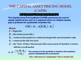
RECAP: CAPM & SML E(return) = Risk-free rate of return + Risk premium specific to asset i = Rf + (Market price of risk)x(quantity of risk of asset i) E(Ri) = Rf + [E(RM)-Rf] x [COV(Ri, RM)/Var(RM)] E(Ri) = Rf + [E(RM)-Rf] x βi E(Ri) SML E(RM) slope = [E(RM) - Rf] = Eqm. Price of risk Rf βi = COV(Ri, RM)/Var(RM) βM = 1
Empirical Studies of CAPM • Is CAPM useful? • Given many unrealistic assumptions, how good does the model fit into the reality? • Think about the following questions: [1] What exactly are the predictions of the CAPM? [2] Are they testable? [3] What is a regression? [4] How to test hypothesis? What is t-test?
[1] What are the predictions ? [a] CAPM says: more risk, more rewards [b] HOWEVER, “reward-able” risk ≠ asset total risk, but = systematic risk (beta) [c] We ONLY need Beta to predict returns [d] return LINEARLY depends on Beta
[2] Testable ? Ideally, we need the following inputs: [a] Risk-free borrowing/lending rate {Rf} [b] Expected return on the market {E(RM)} [c] The exposure to market risk {βi = cov(Ri,RM)/var(RM)} E(Ri) = Rf + [E(RM)-Rf] x [COV(Ri, RM)/Var(RM)] E(Ri) = Rf + [E(RM)-Rf] x βi
[2] Testable ? E(Ri) = Rf + [E(RM)-Rf] x [COV(Ri, RM)/Var(RM)] E(Ri) = Rf + [E(RM)-Rf] x βi In reality, we make compromises: [a] short-term T-bill (not entirely risk-free) {Rf} [b] Proxy of market-portfolio (not the true market) {E(RM)} [c] Historical beta {βi = cov(Ri,RM)/var(RM)}
[2] Testable ? Problem 1: What is the market portfolio? We never truly observe the entire market. We use stock market index to proxy market, but: [i] only 1/3 non-governmental tangible assets are owned by corporate sector. Among them, only 1/3 is financed by equity. [ii] what about intangible assets, like human capital?
[2] Testable ? Problem 2: Without a valid market proxy, do we really observe the true beta? [i] suggesting beta is destined to be estimated with measurement errors. [ii] how would such measurement errors bias our estimation?
[2] Testable ? Problem 3: Borrowing restriction. Problem 4: Expected return measurement. [i] are historical returns good proxies for future expected returns? Ex Ante VS Ex Post
[3] Regression E(Ri) = Rf + [E(RM)-Rf] x [COV(Ri, RM)/Var(RM)] E(Ri) = Rf + [E(RM)-Rf] x βi E(Ri) – Rf= [E(RM)-Rf] x βi With our compromises, we test : [Ri – Rf] = [RM-Rf] x βi Using the following regression equation : [Rit – Rft] = γ0 + γ1βi + εit In words, Excess return of asset i at time t over risk-free rate is a linear function of beta plus an error (ε). Cross-sectional Regressions to be performed!!!
[3] Regression [Rit – Rft] = γ0 + γ1βi + εit CAPM predicts: [a] γ0 should NOT be significantly different from zero. [b] γ1 = (RMt - Rft) [c] Over long-period of time γ1 > 0 [d] β should be the only factor that explains the return [e] Linearity
[4] Generally agreed results [Rit – Rft] = γ0 + γ1βi + εit [a] γ0> 0 [b] γ1 < (RMt - Rft) [c] Over long-period of time, we have γ1 > 0 [d] β may not be the ONLY factor that explains the return (firm size, p/e ratio, dividend yield, seasonality) [e] Linearity holds, β2 & unsystematic risk become insignificant under the presence of β.
[4] Generally agreed results [Rit – Rft] CAPM Predicts Actual γ1= (RMt - Rft) γ0 = 0 βi
Roll’s Critique Message: We aren’t really testing CAPM. Argument: Quote from Fama & French (2004) “Market portfolio at the heart of the model is theoretically and empirically elusive. It is not theoretically clear which assets (e.g., human capital) can legitimately be excluded from the market portfolio, and data availability substantially limits the assets that are included. As a result, tests of CAPM are forced to use compromised proxies for market portfolio, in effect testing whether the proxies are on the min-variance frontier.” Viewpoint: essentially, implications from CAPM aren’t independently testable. We do not have the benchmark market to base on. Every implications are tested jointly with whether the proxy is efficient or not.