Download
1 / 1
10 likes | 82 Views
Further Modeling using the Information Integration Model of Consciousness Michael W. Hadley, Matt McGranaghan , Chun Wai Liew and Elaine R. Reynolds Neuroscience Program and Department of Computer Science, Lafayette College, Easton PA 18042. 687.24 HH42. P. Introduction.

E N D
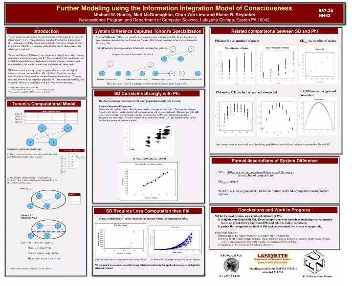
Further Modeling using the Information Integration Model of Consciousness Michael W. Hadley, Matt McGranaghan, Chun WaiLiew and Elaine R. Reynolds Neuroscience Program and Department of Computer Science, Lafayette College, Easton PA 18042 687.24 HH42 P Introduction System Difference Captures Tononi’s Specialization Related comparisons between SD and Phi Tononi proposes a definition of consciousness as “the capacity to integrate information” (1, 2). This capacity is modeled by effective information (EI), a measure of all the causal interactions between two subsets of nodes in a system. Phi (Φ) is a measure of the EI that can be shared across the subsets of a system (3). Tononi and Sporns (2003) used an optimization algorithm to drive random connection matrices towards high Φ. They concluded that two factors lead to high Φ: specialization, a high degree of node structure variance; and connectedness, the ability to reach any node from any other node. We built on their work by trying to capture characteristics of high Φ matrices into our own variables. We calculated Φ and our variable measures over a large, random sample of connection matrices. Then we analyzed how well our variables explained Φ. One particular variable, SD or system difference, correlated well with Φ in various measures. 1 Tononi BMC Neuroscience 2004, 5:42 2 Tononi and Koch (2008) Ann. N.Y. Acad. Sci. 1124: 239–261 3 Tononi and Sporns (2003) BMC Neuroscience 2003, 4:31 System Difference (SD) is our variable that correlates most strongly with Phi. It was based on the specialization characteristic that Tononi and Sporns (2003) found in matrices that were optimized to have high Phi. Phi and SD vs. number of nodes SDavg vs. number of nodes The SD model is based on counting differences in connection patterns. Compare the outputs from node 3 to node 4. Difference in outputs to node 1 No difference in outputs to node 2 Difference in outputs to node 3 No difference in outputs to node 4 Thus, there are a total of 2 differences between the outputs of node 3 and node 4. SD (100 nodes) vs.percent connected Phi and SD (11 nodes) vs. percent connected SD Correlates Strongly with Phi We observed strong correlations with every population sample that we used. Tononi’s Computational Model Random Normalized Population In this trial, the random matrices had the same number of inputs for each node. Each number of inputs from 1 to n-1 had an equal probability of occurring (again self-weights excluded). Matrices had to be fully connected. Isomorphs were detected using the Igraph module for Python. Tononi’s normalization procedure was run, which forces the columns of the matrices to sum to 0.5. The population was further divided into groups by number of nodes. Node 1 Node 2 Node 3 Node 4 Any comparisons we have tried so far (including graph theory metrics) have had similar patterns for Phi and SD The model works in three main steps: 1. The given system is broken into all possible subsets of sizes 2 through n (total number of nodes). 2. The effective information (EI) for each subset is calculated. This is done by finding the minimum EI across all bipartitions of the subset. 3. Phi Φis the maximum of the EIs for the subsets All Possible Subsets 10 Nodes, 12000 Matrices, r=0.8708 Formal descriptions of System Difference SD = Difference of the outputs + Difference of the inputs the number of comparisons SDmax = n2/n-1 We have also have generated a formal definition of the SD computationusingmatrix algebra Subset 1, 2, 3 Conclusions and Work in Progress SD Requires Less Computation than Phi SD shows great promise as a short-cut estimate of Phi. It is highly correlated with Phi. Every comparison were have done including various metrics based on graph theory have found Phi and Sd to be highly correlated It pushes the computational limit of Phi back an estimated two orders of magnitude. Future work includes: Optimization of SD-what properties of a system produce optimum SD Extension of SD to multi-weight systems. The populations used so far have all been for single weight systems, so SD’s explanatory power in multi-weight systems has not been explored. Comparisons of SD in biologically relevant structures. Subset 1, 2, 3 Bipartition 3; 1,2 The major limitation of Tononi’s model is the amount of time the computation takes. EI(A→B) = MI(AHmax:B) MI(A:B) = H(A) + H(B) - H(AB) H(A) = (1/2) ln [ (2π e) n |COV(A)| ] EI(A B) = EI(A→B) + EI(B→A) At just 15 nodes, the processing time forΦis around 3 hours. At 1000 nodes, the SD processing takes under 2 minutes. SD is a much less computationally taxing calculation allowing for application to more biologically relevant systems. Funding provided by NSF IIS-0722211 awarded to CWL FUN Travel Award Winner