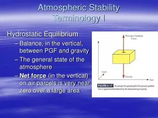
ATMOSPHERIC STABILITY Hydrodynamic stability Parcel method Stability criteria

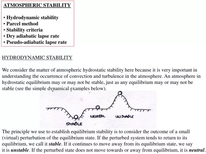
1. ATMOSPHERIC STABILITY • Hydrodynamic stability • Parcel method • Stability criteria • Dry adiabatic lapse rate • Pseudo-adiabatic lapse rate HYDRODYNAMIC STABILITY We consider the matter of atmospheric hydrostatic stability here because it is very important in understanding the occurrence of convection and turbulence in the atmosphere. An atmosphere in hydrostatic equilibrium may or may not be stable, just as any equilibrium may or may not be stable (see the simple dynamical examples below). The principle we use to establish equilibrium stability is to consider the outcome of a small (virtual) perturbation of the equilibrium state. If the perturbed system tends to return to its equilibrium, we call it stable. If it continues to move away from its equilibrium state, we say it is unstable. If the perturbed state does not move towards or away from equilibrium, it is neutral.

2. Notes: 1) If the system returns to equilibrium by decaying oscillations, it is said to have focal stability. If it returns to equilibrium without oscillations, it is said to have nodal stability (A.B. Pippard, 1985: Response and stability, p. 11) 2) In the unstable case, the system may move away from equilibrium continuously, or by ever increasing oscillations. In linear mathematical systems, the amplitude of the perturbation may increase without bound, but in real physical systems, energy considerations generally prevent this, with the result that the system may eventually arrive at a different equilibrium. PARCEL METHOD When applying these notions to the atmosphere, we have to decide how to perturb the hydrostatic equilibrium. Normally, we imagine doing this by defining a small air parcel and considering small vertical displacements of it from its initial location. This is referred to as the parcel method. If the displaced air parcel experiences a restoring force, tending to move it back towards its starting point, we say the equilibrium is stable. If there is no restoring force, we call it neutral. Finally if the displaced parcel experiences a force pushing it further from its starting point, we say the equilibrium is unstable (see the sketches below).

3. In the following description of this method, we will make a few simplifying assumptions. • The air parcel is initially in equilibrium with its environment, so that they have identical • pressure, temperature, and density. The atmosphere initially is in hydrostatic equilibrium. • 2) The pressure in the air parcel is always identical to the pressure in the environment at the • same level as the parcel. If this were not the case, there would be horizontal pressure gradients, • leading to horizontal motion, which is of no immediate interest when considering hydrostatic • stability. • 3) The parcel does not mix with the environment, nor is the environment disturbed by the ascent • of the parcel. • 4) The air parcel is dry, and the vertical displacement is rapid, so that its temperature changes • adiabatically at the dry adiabatic lapse rate, d=g/cp. [Note: if the air parcel is moist (but not • saturated), the parcel temperature should be replaced by the virtual temperature.] STABILITY CRITERIA From the previous sketches, it is easy to see that hydrostatic stability or instability depends on the magnitude of the local environmental lapse rate, relative to the dry adiabatic lapse rate (parcel lapse rate). This result may be summarized as follows: (19.1)

4. We could also define the stability criteria in terms of the potential temperature lapse rate of the environment, relative to the potential temperature lapse rate of the parcel (which is zero for adiabatic changes). Hence: (19.2) If the parcel is saturated, we can obtain the appropriate stability criteria from Eq. 19.1 by replacing the dry adiabatic lapse rate with the pseudo-adiabatic lapse rate, s, on the right hand side. Thus it is important to determine dands. DRY ADIABATIC LAPSE RATE Although we have already quoted an expression for dabove,we will do the derivation here for the sake of completeness. Logarithmically differentiating the definition of potential temperature, we have: (19.3)

5. Multiplying by T, and substituting from the hydrostatic equation and the ideal gas law into the second term on the right hand side (keeping in mind that the vertical pressure gradient in the hydrostatic equation is determined by the environmental density and hence the environmental temperature, Te), leads to: (19.4) PSEUDOADIABATIC LAPSE RATE Recalling that for cloudy air undergoing a reversible adiabatic process, the change in specific entropy is given by Eq. 9.10: (19.5) Differentiating with respect to height, Eq. 19.5 can be re-arranged to give an expression for the pseudoadiabatic lapse rate: (19.6)

6. Differentiating the relationship between saturation mixing ratio and saturation vapour pressure, , and substituting into the first term of Eq. 19.6, then substituting the hydrostatic equation and ideal gas law into the second term of Eq. 19.6, and finally using the chain rule and the Clausius-Clapeyron equation, leads to: (19.7) Since lv/cp1500 K, the denominator in Eq. 19.7 always exceeds the numerator (for meteorological conditions), with the result (which we know already from the tephigram), that sd . The equality arises if the air is dry (rs=0), in which case the ratio in Eq. 19.7 becomes unity. At high pressures and low temperatures, we also have s ~ d (see the tephigram to confirm this).

7. ATMOSPHERIC STABILITY II • Vertical oscillations in a stable atmosphere • Brunt-Väisälä frequency VERTICAL OSCILLATIONS IN A STABLE ATMOSPHERE A stable atmosphere exhibits focal stability. That is, air parcels displaced from equilibrium will return to it by means of decaying oscillations. When friction is small, as in the free atmosphere, the oscillations may continue for a long time. This process is of some intrinsic interest, inasmuch as some internal gravity waves in the atmosphere arise from the oscillation of air parcels displaced from equilibrium by flow over topography. We will calculate the frequency of these oscillations by solving the equation of motion of the displaced air parcel. Since the environment is in hydrostatic equilibrium, by assumption, its equation of motion is simply the hydrostatic equation: (20.1) Where the subscript “e” refers to the environment. Unsubscripted variables will refer to the air parcel. The equation of motion of the air parcel is given by Newton’s second law for a unit mass of air:

8. (20.2) If we assume that the parcel and environmental pressures at the same level are identical, then Eq. 20.2 may be written: (20.3) Substituting from Eq. 20.1 leads to: (20.4) The term on the right hand side is called the buoyancy, and it is clearly positive (leading to upwards acceleration) if the specific volume of the parcel exceeds the specific volume of the environment. It is clearly negative if the parcel’s specific volume is less than that of the environment, and the resulting acceleration will be downwards. Buoyancy is often written (approximately) as gv/v, g/,orgT/T, where the meaning of the deltas can be ascertained by substituting either the ideal gas law or v=1/ into Eq. 20.4. Buoyancy is also sometimes referred to as reduced gravity, for obvious reasons. Since we have Assumed that p=pe, an application of the ideal gas law leads to v/ve=T/Te. This result can be

9. substituted into Eq. 20.4 to give: (20.5) Assuming the parcel displacement is small, we may write: (20.6) where the subscript “0” refers to the initial point of the air parcel. Substituting from Eq. 20.6 into Eq. 20.5, we have, finally: (20.7) BRUNT-VÄISÄLÄ FREQUENCY Eq. 20.7 leads independently to the stability criteria which we fomulated in the previous lecture (see Eqs. 19.1, 19.2). Here, however, we will use it to solve for the frequency of oscillations in the stable case. Note that in form the equation is identical to that describing a spring (with a particular spring constant) undergoing periodic oscillations. Let us assume a solution of the form . Then upon substitution into Eq. 20.7

10. and solving for : (20.8) This quantity is the Brunt-Väisälä period. It is the period of small amplitude, vertical, gravity- controlled oscillations in a stable atmosphere. The Brunt-Väisälä frequency is 1/. By logarithmically differentiating the defining equation for potential temperature, and making use of the hydrostatic equation and the ideal gas law, it may be shown that: (20.9) Hence, the Brunt-Väisälä frequency may also be written as: (20.10) As an example, if e=9oC/km then  ~1000s. In a wind of 10 m/s, the vertical oscillations will give rise to waves of wavelength about 10 km. If the conditions are right, these may be visible as a regular pattern of lenticular clouds, which form in the updraft sections of the waves.

11. Images taken from the website of Bruce Sutherland (http://taylor.math.ualberta.ca/~bruce ) Internal waves over Edmonton (A. Mehta) Internal waves viewed from space. Internal waves launched by flow through Strait of Gibraltar. More internal waves from space.

12. ATMOSPHERIC STABILITY III • Conditional instability • Stability changes caused by lifting air masses • Convective instability CONDITIONAL INSTABILITY Up to this point, we have examined atmospheric hydrostatic stability by considering the virtual, vertical displacement of dry air parcels. But what if they are saturated (I.e., cloudy)? Certainly, the vertical displacement of cloudy air occurs in the atmosphere. A little thought about this problem will quickly lead to the conclusion that the stability criteria for this case are analogous to those for the dry case, except that the parcel’s dry adiabatic lapse rate is replaced by the pseudo-adiabatic lapse rate. Thus, for a saturated atmosphere, the stability criteria are: (21.1) Since s < d it is thus “easier” to obtain instability with saturated air than with dry air. Supposing now that we don’t know whether the virtual parcel of air we displace will be saturated or unsaturated. But we would nevertheless like to say something about the stability of

13. the atmosphere. NOTE: Keep in mind that stability is a property of the atmosphere, not of the virtual parcels of air we choose to displace from their equilibrium. What can we say? If  < s then the atmosphere will be stable for both saturated and unsaturated Parcel displacements. We call this absolute stability. Similarly, if  > d the atmosphere will be Unstable for both saturated and unsaturated parcel displacements. This is absolute instability. If the environmental lapse rate lies between the pseudoadiabatic and the dry adiabatic value, Stability will depend on whether saturated or unsaturated parcel displacement occurs. This is Known as conditional instability. We summarize these results below. NOTE: Conditional instability here, which is a form of static instability, should not be confused with conditional instability of the second kind (CISK), which is a form of dynamic instability occurring in the tropics. CISK arises out of a cooperative interaction (positive feedback) between cumulus convection and a large-scale disturbance. In a hurricane, for example, cumulus convection provides the latent heat energy that is converted into kinetic energy and drives the hurricane winds. In turn, the hurricane provides moisture convergence near the surface, which feeds the cumulus convection. (21.2)

14. The sketch below illustrates what will happen when a parcel of air is lifted through a large vertical displacement in an atmosphere with a conditionally unstable lapse rate. NOTE: Up to this point we have been considering only small vertical displacements of air parcels, and this is all that is needed in order to determine the local stability of the atmosphere. But we know that real atmospheric processes (e.g., convection) lead to large vertical displacement of air parcels. So it is quite realistic to consider the consequences of such displacements. Some physical mechanism will be required to lift the parcel through the stable region. This could be orographic ascent, or ascent arising from a combination of divergence above and convergence below. In the sketch above, the parcel is initially at point A. As it is lifted, it is colder than its environment, so work must be done in order to lift it to the level of free

15. convection (LFC). This work is the negative area on the tephigram and is hatched. After reaching the LFC, the parcel becomes warmer than its environment and continues to rise pseudoadiabatically. The environment now performs work on the parcel, and this is the positive area on the tephigram (also hatched). Part of this work will be required to overcome “friction” as the parcel rises through its environment, and part will be converted into kinetic energy in the updraft of the resulting cloud. NOTE: This is not molecular friction. Much of it is the results of entrainment of ambient air (with low vertical momentum) into the cloud. If you observe closely, you can see how this happens at the edge of a cloud as cloudy elements engulf clear air and drag it into the cloud. Some of it is due to turbulent drag, and finally some of it will be due to the drag of the precipitation particles. If we were to convert all of the positive area into kinetic energy, this would give an upper limit to the maximum possible updraft in the cloud. PROOF: THAT THE WORK REQUIRED TO LIFT AN AIR PARCEL FROM POINT A TO POINT B EQUALS THE NEGATIVE AREA ON THE TEPHIGRAM BETWEEN THE ENVIRONMENT AND PARCEL SOUNDINGS. The work done in lifting a unit mass through the vertical distance from A to B is, from integrating Work=Force  Distance,

16. Substituting from the equation of motion (Eq. 20.4): where the last equality arises from the use of the hydrostatic equation and the ideal gas law (keeping in mind that we are assuming the pressure in the environment equals the pressure in the air parcel at the same level). Making use of the definition of potential temperature, and keeping in mind that the parcel and environmental temperatures are the same at points A and B, we have finally: This is just the negative area on the tephigram, illustrated in the previous sketch. If an air parcel rising from the surface gives rise to a positive area on the tephigram sounding (see sketch below), it is likely that air parcels rising from some finite layer above the surface will also give rise to a positive area. This layer of air near the surface is said to have latent instability. The top of the layer with latent instability occurs at the point where rising parcels cease to produce a positive area on the sounding. Even though there may be a layer with latent instability near the surface, there will be no cumulus cloud formation unless there is some means to produce the work necessary to overcome the lower negative area on the sounding. This may be accomplished by surface

17. heating, which will tend to modify the lowest portion of the sounding, making it dry adiabatic. The convective condensation level (CCL) is the point of intersection of this dry adiabat with an equisaturated curve whose value represents the average mixing ratio over the lowest 50 mb. The convective temperature, Tc, is the surface temperature at the bottom of the dry adiabat, extending downwards from the CCL. It is an estimate of the surface temperature that must be achieved in order to cause the onset of cumulus convection on a particular day.

18. The positive area on a tephigram is often used to predict the intensity (severity) of convection. Since areas are not so easy to measure, various indices have been developed that give a measure of this area. One of the earliest, and still used, is the Showalter Index. It is defined as the difference between the parcel and environment temperatures at 500 mb, for parcels rising from 850mb. STABILITY CHANGES CAUSED BY LIFTING AIR MASSES LIFTING A DRY AIR MASS As an air mass rises or subsides (descends) in the atmosphere, its stability can change as a consequence of changes in its lapse rate (since, as we have seen above, the local lapse rate determines the local stability). We will begin by considering the case of a dry air mass, and examine a layer within it defined by two isobaric surfaces (so that the mass of the layer is fixed). If we use the vertical lapse rate of potential temperature to examine stability (Eq. 19.2), then we need to examine how /z varies during lifting. Since the process is dry, by assumption,  will not change. However, z will increase as a result of expansion of the air mass in the vertical. The result is that the magnitude of the potential temperature gradient will be reduced. Thus, whatever the initial stability, or instability, it will be reduced as lifting moves the lapse rate closer to neutral. Conversely, subsidence in the atmosphere increases stability or instability, by moving the lapse rate further from neutral (z decreases as the air mass is compressed during descent). See the following sketch for an illustration of how this occurs. You may wish to consider an example on the tephigram for yourself.

19. LIFTING AN AIR MASS WHICH BECOMES SATURATED In the three following sketches, we show that when an initially isothermal layer is lifted to a Level where it becomes entirely saturated, its final stability depends on the lapse rate of the Adiabatic equivalent potential temperature (or the adiabatic wet-bulb potential temperature). NOTE: Remember that aeis conserved during adiabatic lifting, so that it doesn’t matter whether we speak of the initial or the final lapse rate of the adiabatic equivalent potential temperature. They are the same. Moreover, you can convince yourself, by considering examples with other initial lapse rates, that the result is independent of the initial temperature lapse rate, and hence independent of the initial stability of the layer.

20. In summary, a layer that is lifted until it is completely saturated has a stability, after lifting, that is independent of its initial stability, but depends on the initial vertical gradient of adiabatic equivalent potential temperature, as follows: (21.3) Just to confuse matters, some people refer to this as potential stability or instability, so be prepared to encounter both names. As an example of the use of this concept, consider orographic flow leading to cloud formation. If the air mass is potentially stable, we would expect stratiform clouds to ensue, and possible steady rainfall. If the air mass is potentially unstable, cumuliform clouds and showers are likely.