Download
1 / 88
890 likes | 1.09k Views
New methods for estimating species trees from gene trees. Tandy Warnow March 12, 2012. Phylogeny (evolutionary tree). Orangutan. Human. Gorilla. Chimpanzee. From the Tree of the Life Website, University of Arizona. -3 mil yrs. AAGACTT. AAGACTT. -2 mil yrs. AAG G C C T. AAGGCCT.

E N D
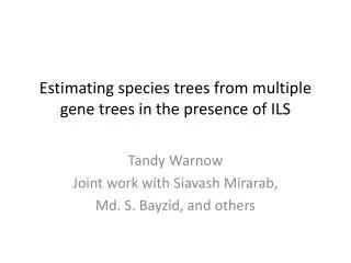
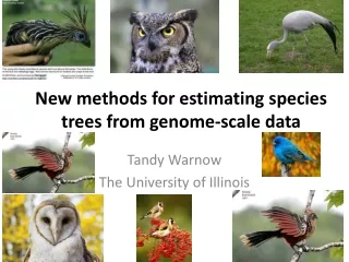
New methods for estimating species trees from gene trees Tandy Warnow March 12, 2012
Phylogeny(evolutionary tree) Orangutan Human Gorilla Chimpanzee From the Tree of the Life Website,University of Arizona
-3 mil yrs AAGACTT AAGACTT -2 mil yrs AAGGCCT AAGGCCT AAGGCCT AAGGCCT TGGACTT TGGACTT TGGACTT TGGACTT -1 mil yrs AGGGCAT AGGGCAT AGGGCAT TAGCCCT TAGCCCT TAGCCCT AGCACTT AGCACTT AGCACTT today AGGGCAT TAGCCCA TAGACTT AGCACAA AGCGCTT AGGGCAT TAGCCCA TAGACTT AGCACAA AGCGCTT DNA Sequence Evolution
Input: unaligned sequences S1 = AGGCTATCACCTGACCTCCA S2 = TAGCTATCACGACCGC S3 = TAGCTGACCGC S4 = TCACGACCGACA
Phase 1: Multiple Sequence Alignment S1 = AGGCTATCACCTGACCTCCA S2 = TAGCTATCACGACCGC S3 = TAGCTGACCGC S4 = TCACGACCGACA S1 = -AGGCTATCACCTGACCTCCA S2 = TAG-CTATCAC--GACCGC-- S3 = TAG-CT-------GACCGC-- S4 = -------TCAC--GACCGACA
Phase 2: Construct tree S1 = AGGCTATCACCTGACCTCCA S2 = TAGCTATCACGACCGC S3 = TAGCTGACCGC S4 = TCACGACCGACA S1 = -AGGCTATCACCTGACCTCCA S2 = TAG-CTATCAC--GACCGC-- S3 = TAG-CT-------GACCGC-- S4 = -------TCAC--GACCGACA S1 S2 S4 S3
Progress on Gene Tree and Alignment Estimation • Statistical performance of phylogeny estimation methods • Co-estimation of alignments and trees (SATé) • “Alignment-free” phylogeny estimation (DACTAL) • Phylogenetic analysis and alignment of NGS data (SEPP) • Taxon identification of short reads from same gene (metagenomic analysis) (TIPP) Tomorrow’s talk will cover SATé, SEPP, and TIPP
Single gene vs. multi-gene analyses • Most methods analyze single genes (or other genomic region). These produce estimated “gene trees”. • But species trees are estimated using multiple genes.
Multi-gene analyses After alignment of each gene dataset: • Combined analysis: Concatenate (“combine”) alignments for different genes, and run phylogeny estimation methods • Supertree: Compute trees on alignment and combine gene trees
gene 1 gene 3 S1 TCTAATGGAA S1 S2 gene 2 GCTAAGGGAA TATTGATACA S3 S3 TCTAAGGGAA TCTTGATACC S4 S4 S4 TCTAACGGAA GGTAACCCTC TAGTGATGCA S7 S5 TCTAATGGAC GCTAAACCTC S7 TAGTGATGCA S8 S6 TATAACGGAA GGTGACCATC S8 CATTCATACC S7 GCTAAACCTC Not all genes present in all species
Two competing approaches gene 1gene 2 . . . gene k . . . Analyze separately . . . Supertree Method Species Combined Analysis
c d a e c d a f b f Constructing trees from subtrees Let T|A denote the induced subtree of T on the leafset A T|{a,c,d,f} T Question: given induced subtrees of T for many subsets of taxa -- can you produce the tree T?
Supertree estimation Challenges: • Tree compatibility is NP-complete (therefore, even if subtrees are correct, supertree estimation is hard) • Estimated subtrees have error Advantages: • Estimating individual gene trees can be computationally feasible (compared to the combined analysis of many genes) • Can use different types of data for each gene
MRP weighted MRP MRF MRD Robinson-Foulds Supertrees Min-Cut Modified Min-Cut Semi-strict Supertree QMC Q-imputation SDM PhySIC Majority-Rule Supertrees Maximum Likelihood Supertrees and many more ... Matrix Representation with Parsimony (Most commonly used and most accurate) Many Supertree Methods
Quantifying topological error c d d a e a c e b f b f • False negative (FN): bB(Ttrue)-B(Test.) • False positive (FP): bB(Test.)-B(Ttrue) True Tree Estimated Tree
FN rate of MRP vs. combined analysis Scaffold Density (%)
SuperFine-boosting: improves accuracy of MRP Scaffold Density (%) (Swenson et al., Syst. Biol. 2012)
SuperFine • First, construct a supertree with low false positives The Strict Consensus • Then, refine the tree to reduce false negatives by resolving each polytomy using a “base” supertree method (e.g., MRP) Quartet Max Cut
Obtaining a supertree with low FP The Strict Consensus Merger (SCM) SCM of two trees Computes the strict consensus on the common leaf set Then superimposes the two trees, contracting more edges in the presence of “collisions”
e b a e c b a f g d f g b a c h d i j c h i j d Strict Consensus Merger (SCM) b e a f c d g a b c h d i j
Performance of SCM • Low false positive (FP) rate (Estimated supertree has few false edges) • High false negative (FN) rate (Estimated supertree is missing many true edges)
Theoretical results for SCM • SCM can be computed in polynomial time • For certain types of inputs, the SCM method solves the NP-hard “Tree Compatibility” problem • All splits in the SCM “appear” in at least one source tree (and project onto each source tree)
Resolving a single polytomy, v, using MRP • Step 1: Reduce each source tree to a tree on leafset, {1,2,...,d} where d=degree(v) • Step 2: Apply MRP to the collection of reduced source trees, to produce a tree t on {1,2,...,d} • Step 3: Replace the star tree at v by tree t
e b a e c b a f g d f g b a c h d i j c h i j d Part 1 of SuperFine b e a f c d g a b c h d i j
b 1 e 1 a 1 1 e b f 6 6 a c 1 d 4 4 g 5 5 f g a b 1 1 c 1 2 3 h d h 1 i j i j 4 5 6 c 1 a c e b h 2 2 3 d g f d 4 4 i j 3 3 Part 2 of SuperFine
Theorem Given • a set of source trees, • SCM tree T, • and a polytomy in T, after relabelling and reducing, each source tree has at most one leaf with each label.
1 4 6 5 1 4 2 3 Step 2: Apply MRP to the collection of reduced source trees 5 1 4 MRP 2 3 6
b e c a e b a f g c h j d i j i i j a c e b Replace polytomy using tree from MRP g 5 d 4 1 2 3 h 6 f h d g f
SuperFine-boosting: improves accuracy of MRP Scaffold Density (%) (Swenson et al., Syst. Biol. 2012)
SuperFine is also much faster MRP 8-12 sec. SuperFine 2-3 sec. Scaffold Density (%) Scaffold Density (%) Scaffold Density (%)
Limitations of Supertree Methods • Traditional supertree methods assume that the true gene trees match the true species tree. • This is known to be unrealistic in some situations, due to processes such as • Deep coalescence (“incomplete lineage sorting”) • Gene duplication and loss • Horizontal gene transfer
Past Present Multiple populations/species Courtesy James Degnan
Gene tree in a species tree Courtesy James Degnan
Deep Coalescence • Population-level process, also called “Incomplete Lineage Sorting” • Gene trees can differ from species trees due to short times between speciation events (population size also impacts this probability) • Causes difficulty in estimating some species trees (such as human-chimp-gorilla)
Phylogeny(evolutionary tree) Orangutan Human Gorilla Chimpanzee From the Tree of the Life Website,University of Arizona
MDC Problem • MDC(minimize deep coalescence) problem: • given set of true gene trees, find the species tree that implies the fewest deep coalescence events • Posed by Wayne Maddison, Syst Biol 1997
Extra Lineages XL(T,t) • T is the species tree • t is the gene tree • XL(T,t): the number of extra lineages, under the best embedding of t into T
Two MDC problems Score pair of trees: • Input: rooted binary gene tree t and species tree T • Output: XL(T,t) Find best species tree: • Input: set X of rooted, binary gene trees on set S • Output: species tree T on S that minimizes XL(T,X) = t XL(T,t).
Limitations of methods for MDC Current methods typically assume • input gene trees are correct, binary, rooted trees containing all the taxa But • Estimated gene trees are usually partially incorrect, are often unrooted, and may not be complete. • Assuming all gene tree incompatibility is due to deep coalescence is likely problematic.
Minimizing Deep Coalescence (MDC) • Than and Nakhleh (PLoS Comp Biol 2009): algorithms for MDC which assume all gene trees are correct, rooted, binary trees. • Yu, Warnow, and Nakhleh (RECOMB 2011 and J Comp Biol 2011) extends T&N 2009 to handle estimated gene trees that are unrootedand have errors. • Bayzid and Warnow (J Comp Biol, in press) extends T&N 2009 to handle incomplete gene trees.
Search: main results in T&N 2009 • Theorem: Let X be a set of k rooted binary gene trees on taxon set S, and let C be a set of subsets of the taxon set. Then a species tree T that optimizes MDC with Clusters(T) C can be found in time that is polynomial in |C|, n, and k. • Exact MDC: Let C be all possible subsets of S • “Heuristic” MDC: Let C be the set of “clusters” of the input gene trees (where a cluster is the set of leaves below a node in a tree)
T&N 2009: B-maximal clusters and kB(t) T is a species tree, and t is a gene tree, both rooted and binary Definitions • B is a cluster of T • Y is a B-maximal cluster in t if (i) Y is a cluster of t, (ii) Y B, and (iii) Y Z for any other cluster Z of t such that Z B. • kB(t) is the number of B-maximal clusters in t
Calculating XL(T,t) Lemma (T&N 2009): Let T be a binary species tree and t be a binary rooted gene tree. Then for an optimal embedding of t into T: • kB(t) is the number of lineages on the edge “above” subtree for B in T • XL(T,t) = B[kB(t)-1], where B ranges over the clusters of T.
Calculating XL(T,X) Define CostB(t)= kB(t)-1, and therefore XL(T,t) = B CostB(t) Given set X of gene trees, define XL(T,X) = t XL(T,t) = t B CostB(t) = B t CostB(t) = B w(B) where w(B) = t CostB(t)
Graph Algorithm for MDC Graph G(X): • Vertex set: v corresponds to non-trivial S(v) S, where S(v) is the cluster of T below node v • Edges: (v,w) present iff clusters S(v) and S(w) can co-exist as clusters in a tree • Vertex weight: Weight(v) =∑t CostS(v)(t) Theorem: T, binary rooted tree on S s.t. XL(T,X)=W, iff (n-2)-clique in G(X) of weight W, where |S|=n. Hence, MDC can be solved by finding a (n-2)-clique of minimum total weight in G(X).
T&N algorithm for MDC • Because of the structure of the graph, we can find a min cost max clique (of size n-2) in polynomial time (in the size of the graph), using dynamic programming. But the graph has 2n vertices! • However, if we constrain the set C of permitted clusters for the species tree, we can find an optimal constrained solution in O(|C|2 nk) time (the “heuristic” algorithm in T&N 2009).
Yu, Warnow and Nakhleh (2011) • Allows for error in estimated gene trees. • RECOMB 2011 and J Comp Biol 2011
Yu, Warnow and Nakhleh (2011) Modify gene trees to reduce false positive error: • Unroot trees • Use bootstrap (or other statistical techniques) to identify the edges that are potentially incorrect • Contract the low support edges Result: estimated gene trees that are likely to be unrooted contractions of the true gene tree.
New MDC problem • Input: set X ={t1, t2, …, tk} of incompletely resolved, unrooted gene trees. • Output: set X’={t’1, t’2, …, t’k} (such that each t’i is a resolved, rooted version of ti, i=1,2…k) and species tree T that minimizes XL(T,X’). In other words, we treat ti as a constraint on the true gene tree for gene i.