Download
1 / 39
420 likes | 764 Views
Descriptive and inferential statistics. Confidence interval. Georgi Iskrov, MBA, MPH, PhD Department of Social Medicine. Outline. Descriptive statistics Measures of central tendency Measures of spread Normal distribution Central limit theorem Outliers Inferential statistics

E N D
Descriptive and inferential statistics.Confidence interval Georgi Iskrov, MBA, MPH, PhD Department of Social Medicine
Outline • Descriptive statistics • Measures of central tendency • Measures of spread • Normal distribution • Central limit theorem • Outliers • Inferential statistics • Confidence interval
Population vs Sample • Population includes all objects of interest, whereas sample is only a portion of the population. • Parameters are associated with populations and statistics with samples. • Parameters are usually denoted using Greek letters (μ, σ), while statistics are usually denoted using Roman letters (x, s).
Descriptive vs Inferential statistics • We compute statistics and use them to estimate parameters. • The computation is the first part of the statistical analysis (Descriptive Statistics) and the estimation is the second part (Inferential Statistics). • Descriptive Statistics The procedure used to organise and summarise masses of data. • Inferential Statistics The methods used to find out something about a population, based on a sample.
Inferential statistics Sampling Population Parameters From population to sample Sample Statistics From sample to population Inferential statistics
Descriptive statistics Descriptive statistics: • Organising data • Tables • Graphs • Summarising data • Central tendency (location) • Variation (spread)
Descriptive statistics Descriptive statistics: • Organising data • Tables • Frequency distributions • Relative frequency distributions • Graphs • Bar chart • Histogram • Boxplot
Frequency distribution Frequency distribution of survival for both groups Survival Frequency 14 2 17 1 21 1 22 2 23 1 24 2 25 1 27 1 28 1 29 1 31 1 33 1 34 2 35 1 39 1 41 1 Total 20 Experimental group (10 patients) Individual survival in months: 23 27 17 34 41 28 22 33 29 14 Classesofvalues Control group (10 patients) Individual survival in months: 24 31 39 35 34 24 14 21 25 22
Relative frequency distribution Relative frequencydistribution of survival for both groups Survival Frequency Percent Cumulative percent 14 2 10% 10% 17 1 5% 15% 21 1 5% 20% 22 2 10% 30% 23 1 5% 35% 24 2 10% 45% 25 1 5% 50% 27 1 5% 55% 28 1 5% 60% 29 1 5% 65% 31 1 5% 70% 33 1 5% 75% 34 2 10% 85% 35 1 5% 90% 39 1 5% 95% 41 1 5% 100% Total 20 100%
Grouped relative frequency distribution Relative frequency distribution of survival for both groups Survival Frequency Percent Cumulative Percent 10 – 14 2 10% 10% 15 – 19 1 5% 15% 20 – 24 6 30% 45% 25 – 29 4 20% 65% 30 – 34 4 20% 85% 35 – 39 2 10% 95% 40 – 44 1 5% 100% Total 24 100% Classesofintervals Whatrulestofollowwhengrouppingdata?
Descriptive statistics Summarising data: • Central tendency (or sample’s middle value) • Mean • Median • Mode • Spread (or summary of differences within groups) • Range • Interquartile range • Variance • Standard deviation
Mean • Most commonly called average. Experimental group (10 patients) Individual survival in months: 23 27 17 34 41 28 22 33 29 14 Experimental group (10 patients) Individual survival in months: 23 27 17 34 41 28 22 33 29 14 Control group (10 patients) Individual survival in months: 24 31 39 35 34 24 14 21 25 22
Mean • Mean is the balance point. • Means can beheavily affected by outliers (data points with extreme values unlike the rest). • Outliers can make the mean a bad measure of central tendency or common experience.
Median • The middle value when a variable’s values are ranked in order. • The point that divides a distribution into two equal halves. • When data are listed in order, the median is the point at which 50% of the cases are above and 50% below it. • The 50th percentile.
Control group (10 patients) Individual survival in months: 14 21 22 24 24 25 31 34 35 39 Median Median = 24.5 (five cases above, five below)
Median • The median is unaffected by outliers, making it a better measure of central tendency, better describing the “typical person” than the mean when data are skewed. • If the recorded values for a variable form a symmetric distribution, the median and mean are identical. • In skewed data, the mean lies further toward the skew than the median.
Mode • The most common data point is called the mode. • Individual survival data for the control group are: 14, 21, 22, 24, 24, 25, 31, 34, 35, 39 • It is possible to have more than one mode. • Ifallvaluesareunique, thereisnomode. • Mode may mot be at the center of a distribution.
Mode • It may give you the most likely experience rather than the typical or central experience. • In symmetric distributions, the mean, median and mode are the same. • In skewed data, the mean and median lie further toward the skew than the mode. Skewed Symmetric Mean Median Mode Mode Median Mean
Spread • Variation of the recorded values on a variable. • The larger the spread, the further the individual cases are from the mean. • The smaller the spread, the closer the individual scores are to the mean. Mean Mean
Range • The spread, or the distance, between the lowest and highest values of a variable. • To get the range for a variable, you subtract its lowest value from its highest value. Experimental group (10 patients) Individual survival in months: 23 27 17 34 4128 22 33 29 14 Range = 41 – 14 = 27 Control group (10 patients) Individual survival in months: 24 31 39 35 34 24 14 21 25 22 Range = 39 – 14 = 25
Standard deviation • Standard deviation takes into account all individual deviations. • A deviation is the distance away from the mean of a case’s score. • Experimental group’s SD = 8.13 months • Control group’s SD = 7.64 months
Standard deviation • The larger standard deviation, the greater amounts of variation around the mean. • Standard deviation is equal to 0, only when all values are the same. • Like the mean, the standard deviation will be inflated by an outlier case value.
Interquartile range • The interquartile range (IQR) is a measure of variability, based on dividing a data set into quartiles. • Quartiles divide a rank-ordered data set into four equal parts. The values that divide each part are called the first, second, and third quartiles; and they are denoted by Q1, Q2, and Q3, respectively. • IQR is equal to Q3 minus Q1.
Central tendency and spread • Central tendency: Mean, mode and median • Spread: Range, interquartile range, standard deviation • Mistakes: • Focusing on only the mean and ignoring the variability • Standard deviation and standard error of the mean • Variation and variance • What is best to use in different scenarios? • Symmetrical data: mean and standard deviation • Skewed data: median and interquartile range
Important rules • When a constant is added to every observation, the new sample mean is equal to original mean plus the constant. • When a constant is added to every observation, the standard deviation is unaffected. • When every observation is multiplied by the same constant, the new sample mean is equal to original mean multiplied by the constant. • When every observation is multiplied by the same constant, the new sample standard deviation is equal to original standard deviation multiplied by the magnitude of the constant.
Normal (Gaussian) distribution • Mean and standard deviations are a particularly appropriate summary for data whose histogram approximates a normal distribution (the bell-shaped curve). • If you say that a set of data has a mean survival of 29 months, the typical listener will picture a bell-shaped curve centered with its peak at 29 months.
Rule of 3-sigma • When data are approximately normally distributed: • approximately 68% of the data lie within one SD of the mean; • approximately 95% of the data lie within two SDs of the mean; • approximately 99% of the data lie within three SDs of the mean.
Normal (Gaussian) distribution • Central limit theorem: • Create a population with a known distribution that is not normal; • Randomly select many samples of equal size from that population; • Tabulate the means of these samples and graph the frequency distribution. • Central limit theorem states that if your samples are large enough, the distribution of the means will approximate a normal distribution even if the population is not Gaussian. • Mistakes: • Normal vs common (or disease free); • Few biological distributions are exactly normal.
Outliers • Values that lie very far away from the other values in the data set.
Outliers • Outliers can occur for several reasons: • Invalid data entry • Biological diversity • Random chance • Experimental error • Skewed distribution • Mistakes: • Not realizing that outliers are common in data sampled from skewed distribution • Eliminating outliers only when you do not get the results you want
Outliers • Outlier test: • If values are sampled from a normal distribution, what is the chance one value will be as far from the others as the extreme value observed? • Examples: Chauvenetcriterion, Grubbs test, Peirce criterion • Nevertheless, deletion of outlier data is generally a controversial practice!
Inferential statistics Sampling Population Parameters From population to sample Sample Statistics From sample to population Inferential statistics
Confidence interval for the population mean Population mean:point estimate vs interval estimate Standard error of the mean – how close the sample mean is likely to be to the population mean. Assumptions: a random representative sample, independent observations, the population is normally distributed (at least approximately). Confidence interval depends on: sample mean, standard deviation, sample size, degree of confidence. Mistakes: 95% of the values lie within the 95% CI; A 95% CI covers the mean ± 2 SD.
Standard error of mean • The sample mean estimates individual values. The uncertainty with which this mean estimates individual values is given by the standarddeviation. • The sample mean estimates the population mean. The uncertainty with which this mean estimates the population mean is given by the standarderrorofthemean.
Confidence interval for the population mean • The confidence interval for the mean gives us a range of values around the mean where we expect the “true” population mean is located. • 95% confidence interval for thepopulation mean is:
The duration of time from first exposure to HIV infection to AIDS diagnosis is called the incubation period. The incubation periods (in years) of a random sample of 30 HIV infected individuals are: 12.0, 10.5, 9.5, 6.3, 13.5, 12.5, 7.2, 12.0, 10.5, 5.2, 9.5, 6.3, 13.1, 13.5, 12.5, 10.7, 7.2, 14.9, 6.5, 8.1, 7.9, 12.0, 6.3, 7.8, 6.3, 12.5, 5.2, 13.1, 10.7, 7.2. Calculate the 95% CI for the population mean incubation period in HIV. X = 9.5 years; SD = 2.8 years SEM = 0.5 years 95% level of confidence => Z = 1.96 µ = 9.5 ± (1.96 x 0.5) = 9.5 ± 1 years 95% CI for µ is (8.5; 10.5 years) Confidence interval for the population mean
X = 9.5 years; SD = 2.8 years SEM = 0.5 years 95% level of confidence => Z = 1.96 µ = 9.5 ± (1.96 x 0.5) = 9.5 ± 1 years 95% CI for µ is (8.5; 10.5 years) 99% level of confidence => Z = 2.58 µ = 9.5 ± (2.58 x 0.5) = 9.5 ± 1.3 years 99% CI for µ is (8.2; 10.8 years) Confidence interval for the population mean
Describing qualitative data • Standard error of proportion: • The 95% confidence interval for a population proportion is: