Download
1 / 21
210 likes | 433 Views
Rotating solid. Euler predicted free nutation of the rotating Earth in 1755 Discovered by Chandler in 1891 Data from International Latitude Observatories setup in 1899 . Monthly data, t = 1 month. Work with complex-values, Z(t) = X(t) + iY (t).

E N D
Rotating solid Euler predicted free nutation of the rotating Earth in 1755 Discovered by Chandler in 1891 Data from International Latitude Observatories setup in 1899
Monthly data, t = 1 month. Work with complex-values, Z(t) = X(t) + iY(t). Compute the location differences, Z(t), and then the finite FT dZT() = t=0T-1exp {-it}[Z(t+1)-Z(t)] Periodogram IZZT() = (2T)-1|dZT()|2
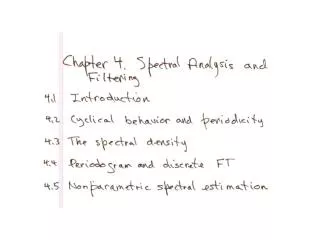
4.3 Spectral distribution function Cp. rv’s
fis non-negative, symmetric(, periodic) White noise. (h) = cov{xt+h,xt} = w2 h=0 and otherwise = 0 f() = w2
dF()/d = f() if differentiable dF() = f()d
Dirac delta function, () a generalized function simplifies many t.s. manipulations r.v. X Prob{X = 0} = 1 P(x) = Prob{X x} = 1 if x 0 = 0 if x < 0 = H(x) Heavyside E{g(X)} = g(0) = g(x) dP(x) = g(x) (x) dx (x) density function = dH(x)/dx
Approximant X N(0,2 ) (x/)/ with small E{g(X)} g(0) cov{dZ(1),dZ(2)} = (1 – 2) f(1) d 1 d 2 Means 0 cov{X,Y} = E{X conjg(Y)} var{X} = E{|X|2}
Periodogram “sample spectral density” Mean“correction”
Non parametric spectral estimation. L = 2m+1


![[PDF] Free Download Whisper Network By Chandler Baker](https://cdn4.slideserve.com/8372276/slide1-dt.jpg)