Download

1 / 144
1.48k likes | 2.07k Views
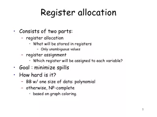
Topic 6 Register Allocation. Revisiting A Typical Optimizing Compiler. Intermediate Language. Front End. Back End. Source Program. Scheduling. Register Allocation. Rationale for Separating Register Allocation from Scheduling.

E N D
Revisiting A Typical Optimizing Compiler Intermediate Language Front End Back End Source Program Scheduling Register Allocation
Rationale for Separating Register Allocation from Scheduling • Each of Scheduling and Register Allocation are hard to solve individually, let alone solve globally as a combined optimization. • So, solve each optimization locally and heuristically “patch up” the two stages.
Why Register Allocation? • Storing and accessing variables from registers is much faster than accessing data from memory. The way operations are performed in load/store (RISC) processors. • Therefore, in the interests of performance—if not by necessity—variables ought to be stored in registers. • For performance reasons, it is useful to store variables as long as possible, once they are loaded into registers. • Registers are bounded in number (say 32.) • Therefore, “register-sharing” is needed over time.
The Goal • Primarily to assign registers to variables. • However, the allocator runs out of registers quite often. • Decide which variables to “flush” out of registers to free them up, so that other variables can be bought in. This important indirect consequence of allocation is referred to as spilling.
Register Allocation and Assignment Allocation: identifying program values (virtual registers, live ranges) and program points at which values should be stored in a physical register. Program values that are not allocated to registers are said to be spilled. Assignment: identifying which physical register should hold an allocated value at each program point.
Live Ranges Live range of virtual register a = (BB1, BB2, BB3, BB4, BB5, BB6, BB7). Def-Use chain of virtual register a = (BB1, BB3, BB5, BB7). a :=... BB1 BB2 T F := a BB3 BB4 := a BB5 BB6 := a BB7
Computing Live Ranges Using data flow analysis, we compute for each basic block: • In the forward direction, the reaching attribute. A variable is reaching block i if a definition or use of the variable reaches the basic block along the edges of the CFG. • In the backward direction, the liveness attribute. A variable is live at block i if there is a direct reference to the variable at block i or at some block jthat succeeds i in the CFG, provided the variable in question is notredefined in the interval between i and j.
Computing Live Ranges (Contd.) The live range of a variable is the intersection of basic- blocks in CFG nodes in which the variable is live, and the set which it can reach.
Local Register Allocation • Perform register allocation one basic block (or super-block or hyper-block) at a time • Must note virtual registers that are live on entry and live on exit of a basic block - later perform reconciliation • During allocation, spill out all live outs and bring all live ins from memory • Advantage: very fast
Local Register Allocation - Reconciliation Codes • After completing allocation for all blocks, we need to reconcile differences in allocation • If there are spare registers between two basic blocks, replace the spill out and spill in code with register moves
Linear Scan Register Allocation • A simple local allocation algorithm • Assume code is already scheduled • Build a linear ordering of live ranges (also called live intervals or lifetimes) • Scan the live range and assign registers until you run out of them - then spill
Linear Scan RA live ranges sorted according to the start time of the first def scan order may use same physical register!
The Linear Scan Algo Source: M. Poletto & V. Sarkar., “Linear Scan Register Allocation”, ACM TOPLAS, Sep 1999. actual spill
Combining Local IS and RA • J.R. Goodman, and W.-C. Hsu, “Code Scheduling and Register Allocation in Large Basic Blocks”, 1988 • Recall phase ordering problem • One solution: combined IS and RA
The Goodman & Hsu Algo • While ready set is not empty do: • if we are not “running out” of registers • select a node from the ready set based on some scheduling priority and mark it as ready (plain list scheduling) • decrease free register count by 1 if instruction writes to a register • if the instruction ends some live ranges, return register to free register pool • else • select the ready node that will free up the most register; and do the same as above • if no such instruction exist, spill! (similar to linear scan)
Global Register Allocation • Local register allocation does not store data in registers across basic blocks. Local allocation has poor register utilization global register allocation is essential. • Simple global register allocation: allocate most “active” values in each inner loop. • Full global register allocation: identify live ranges in control flow graph, allocate live ranges, and split ranges as needed. Goal: select allocation so as to minimize number of load/store instructions performed by optimized program.
Topological Sorting • Given a directed graph, G = V, E, we can define a topological ordering of the nodes • Let T = {v1, v2, ..., vn} be an enumeration of the nodes of V, T is a topological ordering if vi vjE, then i < j (i.e. vi comes before vj in T) • A topological order linearizes a partial order
Global Linear Scan RA • Ignoring back-edges, perform a topological sort of the basic blocks using the CFG • Compute the live range over the entire topological order
Global Live Ranges B1 Topological Order A B1 B2 B3 B4 B2 B3 A B A B B4 B A Global Live Ranges
Simple Example of Global Register Allocation Live range of a = {B1, B3} Live range of b = {B2, B4} No interference! a and b can be assigned to the same register Control Flow Graph a =... B1 T F B2 b = ... ..= a B3 .. = b B4
Second Chance Bin-packing • O. Traub, G. Holloway, and M.D. Smith, “Quality and Speed in Linear-Scan Register Allocation”, SIGPLAN ‘98 • Considers “holes” in live ranges • Considers register allocation as a bin-packing problem • Performs register allocation and spill code generation at the same time
Bin-packing • The binpacking problem: determine how to put the most objects in the least number of fixed space bins • More formally, find a partition and assignment of a set of objects such that constraint is satisfied or an objective function is minimized (or maximized) • In register allocation, the constraint is that overlapping live ranges cannot be assigned to the same bin (register) • Another way of looking at linear scan
Working with holes • We can allocate two non-overlapping live ranges to the same physical register • We can assign two live ranges to the same physical register if one fits entirely into the hole of another
Second Chance Linear Scan • Suppose we encounter variable t, and we assigned a register to it by spilling out variable u currently occupying that register • When u is needed again, it may be loaded into a different register (it gets a “second chance”) • It will stay till its lifetime ends or it is evicted again
A Problem resolution code
Execution Frequency & Global Register Allocation Live range of a = {B1, B2, B3, B4} Live range of b = {B2, B4} Live range of c = {B3} In this example, a and c interfere, and c should be given priority because it has a higher usage count. Control Flow Graph a =... B1 T F B2 b = ... c = c +1 B3 F T ...= a +b B4
Cost and Savings Compilation Cost: running time and space of the global allocation algorithm. Execution Savings: cycles saved due to register residence of variables in optimized program execution. Contrast with memory-residence which leads to longer execution times.
Interference Graph Definition: An interference graphG is an undirected graph with the following properties: (a) each node x denotes exactly one distinct live range X, and (b) an edge exists between nodes x and y iff X Y , where X and Y are the live ranges corresponding to nodes x and y.
Interference Graph Example Live Ranges Interference Graph a Live ranges overlap and hence interfere a := … b := … c := … := a := b d := … := c := d c b Node model live ranges d
The Classical Approach “Register Allocation and Spilling via Graph Coloring”, G. Chatin, Proceedings SIGPLAN-82 Symposium on Compiler Construction, 98-105, 1982. “Register Allocation via Coloring”, G. Chaitin, M. Auslander, A. Chandra, J. Cocke, M. Hopkins and P. Markstein, Computer Languages, vol. 6, 47-57, 1981. more…
The Classical Approach (Contd.) • These works introduced the key notion of an interference graph for encoding conflicts between the live ranges. • This notion was defined for the global control flow graph. • It also introduced the notion of graphcoloring to model the idea of register allocation.
Execution Time and Spill-cost Spilling: Moving a variable that is currently register resident to memory when no more registers are available, and a new live-range needs to be allocated one spill. Minimizing Execution Cost: Given an optimistic assigment— i.e., one where all the variables are register-resident, minimizing spilling.
Graph Coloring • Given an undirected graph G and a set of k distinct colors, compute a coloring of the nodes of the graph i.e., assign a color to each node such that no twoadjacent nodes get the same color. Recall that two nodes are adjacent iff they have an edge between them. • A given graph might not be k-colorable. • In general, it is a computationally hard problem to color a given graph using a given number k of colors. • The register allocation problem uses good heuristics for coloring.
Register Allocation as Coloring • Given k registers, interpret each register as a color. • The graph G is the interference graph of the given program. • The nodes of the interference graph are the executable live ranges on the target platform. • A coloring of the interference graph is an assignment of registers (colors) to live ranges (nodes). • Running out of colors implies not enough registers and hence a need to spill in the above model.
The Approach Discussed Here “The Priority Based Coloring Approach to Register Allocation”, F. Chow and J. Hennessey, ACM Transactions on Programming Languages and Systems, vol. 12, 501-536, 1990.
Important Modeling Difference • The first difference from the classical approach is that now, we assume that the “home location” of a live range is in memory. • Conceptually, values are always in memory unless promoted to a register; this is also referred to as the pessimistic approach. • In the classical approach, the dual of this model is used where values are always in registers except when spilled; recall that this is referred to as the optimistic approach. more...
Important Modeling Difference • A second major difference is the granularity at which code is modeled. • In the classical approach, individual instructions are modeled whereas • Now, basic blocks are the primitive units modeled as nodes in live ranges and the interference graph. • The final major difference is the place of the register allocation in the overall compilation process. • In the present approach, the interference graph is considered earlier in the compilation process using intermediate level statements; compiler generated temporaries are known. • In contrast, in the previous work the allocation is done at the level of the machine code.
The Main Information to be Used by the Register Allocator • For each live range, we have a bit vector LIVE of the basic blocks in it. • Also we have INTERFERE which gives for the live range, the set of all other live ranges that interfere with it. • Recall that two live ranges interfere if they intersect in at least one (basic-block). • If INTERFERE is smaller than the number of available of registers for a node i, then i is unconstrained; it is constrained otherwise. more...
The Main Information to be Used by the Register Allocator • An unconstrained node can be safely assigned a register since conflicting live ranges do not use up the available registers. • We associate a (possibly empty) set FORBIDDEN with each live range that represents the set of colors that have already been assigned to the members of its INTERFERENCE set. The above representation is essentially a detailed interference graph representation.
Prioritizing Live Ranges In the memory bound approach, given live ranges with a choice of assigning registers, we do the following: • Choose a live range that is “likely” to yield greater savings in execution time. • This means that we need to estimate the savings of each basic block in a live range.
Estimate the Savings Given a live range X for variable x, the estimated savings in a basic block i is determined as follows: 1. First compute CyclesSaved which is the number of loads and stored of x in i scaled by the number of cycles taken for each load/store. 2. Compensate the single load and/or store that might be needed to bring the variable in and/or store the variable at the end and denote it by Setup. Note that Setup is derived from a single load or store or a load plus a store. more...
Estimate the Savings (Contd.) 3. Savings(X,i) = {CyclesSaved-Setup} These indicate the actual savings in cycles after accounting for the possible loads/stores needed to move x at the beginning/end of i. 4. TotalSavings(X) = iXSavings(X,i) x W( i ). (a) x is the set of all basic blocks in the live range of X. (b) W( i ) is the execution frequency of variable x in block i. more...
Estimate the Savings (Contd.) 5. Note however that live regions might span a few blocks but yield a large savings due to frequent use of the variable while others might yield the same cumulative gain over a larger number of basic blocks. We prioritize the former case and define: {Priority(X) = TotalSavings(X)/Span(X)} where Span(X) is the number of basic blocks in X.
The Algorithm For all constrained live ranges, execute the following steps: 1. Compute Priority(X) if it has not already been computed. 2. For the live range X with the highest priority: (a) If its priority is negative or if no basic block i in X can be assigned a register—because every color has been assigned to a basic block that interferes with i — then delete X from the list and modify the interference graph. (b) Else, assign it a color that is not in its forbidden set. (c) Update the forbidden sets of the members of INTERFERE for X’. more...
The Algorithm (Contd.) 3. For each live range X’ that is in INTERFERE for X’ do: (a) If the FORBIDDEN of X’ is the set of all colors i.e., if no colors are available, SPLIT (X’). Procedure SPLIT breaks a live range into smaller live ranges with the intent of reducing the interference of X’ it will be described next. 4. Repeat the above steps till all constrained live ranges are colored or till there is no color left to color any basic block.
The Idea Behind Splitting • Splitting ensures that we break a live range up into increasingly smaller live ranges. • The limit is of course when we are down to the size of a single basic block. • The intuition is that we start out with coarse-grained interference graphs with few nodes. • This makes the interference node degree possibly high. • We increase the problem size via splitting on a need-to basis. • This strategy lowers the interference.
The Splitting Strategy A sketch of an algorithm for splitting: 1. Choose a split point. Note that we are guaranteed that X has at least one basic block i which can be assigned a color i.e., its forbidden set does not include all the colors. The earliest such in the order of control flow can be the split point. 2. Separate the live range X into X1 and X2 around the split point. 3. Update the sets INTERFERE for X1 and X2 and those for the live ranges that interfered with X more...
The Splitting Strategy (Contd.) 4. Recompute priorities and reprioritize the list. Other bookkeeping activities to realize a safe implementation are also executed.