Download
1 / 41
410 likes | 622 Views
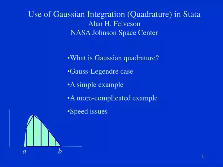
a b. Use of Gaussian Integration (Quadrature) in Stata Alan H. Feiveson NASA Johnson Space Center. What is Gaussian quadrature? Gauss-Legendre case A simple example A more-complicated example Speed issues. 1. What is Gaussian quadrature ?. Wish to evaluate.

E N D
a b Use of Gaussian Integration (Quadrature) in Stata Alan H. Feiveson NASA Johnson Space Center • What is Gaussian quadrature? • Gauss-Legendre case • A simple example • A more-complicated example • Speed issues 1
What is Gaussian quadrature ? Wish to evaluate • Represent H(x) as the product H(x) = W(x) f(x) • Use the approximation where the xj and wj depend on W, a and b.
What is Gaussian quadrature ? • Choose W(x) such that f(x) is “smooth”
What is Gaussian quadrature ? • Choose W(x) such that f(x) is “smooth” • f(x) approximated by linear comb. of orthogonal polynomials {Pj(x)}: Pi(x)Pj(x)dx = 0 (i j ).
What is Gaussian quadrature ? • Choose W(x) such that f(x) is “smooth” • f(x) approximated by linear comb. of orthogonal polynomials {Pj(x)}: Pi(x)Pj(x)dx = 0 (i j ). • xj are zeros of PM(x).
What is Gaussian quadrature ? • Choose W(x) such that f(x) is “smooth” • f(x) approximated by linear comb. of orthogonal polynomials {Pj(x)}: Pi(x)Pj(x)dx = 0 (i j ). • xj are zeros of PM(x). • wj is a weight that depends on
Some types of Gaussian quadrature W(x) = 1 (a ,b) = (any): Gauss-Legendre quadrature W(x) = xe-x (a, b) = (0, ): Gauss-Laguerre quadrature W(x) = (a,b) = (–, ): Gauss-Hermite quadrature
Example 1: -xtlogit- Likelihood at each positive outcome is Estimate by maximum likelihood
Likelihood at each positive outcome is The integrand H(x) = where f(x) is “smooth” H(x) f(x) Example 1: -xtlogit-
W(x) = 1 (a ,b) = (any): Gauss-Legendre quadrature W(x) = xe-x (a, b) = (0, ): Gauss-Laguerre quadrature W(x) = (a,b) = (–, ): Gauss-Hermite quadrature • Example 1: -xtlogit- (cont.) • Maximum likelihood • Likelihood at each obs. is of the form • The integrand is where f(x) is “smooth”
W(x) = 1 (a ,b) = (any): Gauss-Legendre quadrature W(x) = xe-x (a, b) = (0, ): Gauss-Laguerre quadrature W(x) = (a,b) = (–, ): Gauss-Hermite quadrature • Example 1: -xtlogit- (cont.) • Maximum likelihood • Likelihood at each obs. is of the form • The integrand is where f(x) is “smooth” • Uses Gauss-Hermite quadrature see p. 139 (-xtlogit-) and pp. 9 – 14 (-quadchk-)
H(x) f(x) W(x) f(x) • Example 2: Wish to evaluate Let W(x) = Then (Gauss-Laguerre quadrature)
Use of Gaussian Integration (Quadrature) in Stata • What is Gaussian quadrature? • Gauss-Legendre case • A simple example • A more-complicated example • Speed issues 13
Gauss-Legendre Case( W(x) = 1 ) Standard form General form
.6 .4 .2 A B C D E 0 A B C D E -.2 -2 -1 0 1 2 3 x Gauss-Legendre quadrature abcissas and weights –5th order
Use of Gaussian Integration (Quadrature) in Stata • What is Gaussian quadrature? • Gauss-Legendre case • A simple example • A more-complicated example • Speed issues
= norm(3) – norm(0) in Stata A simple example A = 0.4986500740
= norm(3) – norm(0) in Stata A = 0.4986500740 = 0.4986490676 A simple example
= norm(3) – norm(0) in Stata A = 0.4986500740 = 0.4986490676 A simple example . range x 0 3 `K’ . gen fx = normd(x) . integ fx x A = 0.4986489713 (K=26)
Use of Gaussian Integration (Quadrature) in Stata • What is Gaussian integration? • Gauss-Legendre case • A simple example • A more-complicated example • Speed issues
A more-complicated example (cont.) Nonlinear regression Model: yi = F(xi) + ei ei ~ N(0, 2) = ibeta(p, q, x)
Incorporation of M-th order Gaussian quadrature abcissas and weights to data set Contains data obs: 50 vars: 14 size: 4,800 (99.9% of memory free) ------------------------------------------------------------------------------- storage display value variable name type format label variable label ------------------------------------------------------------------------------- y float %9.0g x float %9.0g a float %9.0g lower limit b float %9.0g upper limit u1 double %10.0g abcissa #1 u2 double %10.0g abcissa #2 u3 double %10.0g abcissa #3 u4 double %10.0g abcissa #4 u5 double %10.0g abcissa #5 w1 double %10.0g weight #1 w2 double %10.0g weight #2 w3 double %10.0g weight #3 w4 double %10.0g weight #4 w5 double %10.0g weight #5 -------------------------------------------------------------------------------
program nlgtest version 8.2 /* ---------- Initialization section ------------ */ args y x np a b if "`1'" == "?" { global NP = `np'/* no. of integration points */ global S_1 "P Q " global P=1 /* initialization (poor) */ global Q=1 /* same as above */ /* initialize Gaussian integration variables */ forv i=1(1)$NP { cap gen double lnf`i'=. /* log f(p,q,u_i) */ cap gen double wf`i'=. /* w_i*f(p,q,u_i) */ /* merge Gaussian abcissas (u_i) and weights (w_i) */ run gaussrow _u w $NP `a’ `b’ u } exit }
/* ---------- Iteration section ------------ */ local np = $NP forv i=1(1)`np' { /* loop over quadrature points */ qui replace lnf`i'=lngamma($P+$Q)-lngamma($P)-lngamma(Q) /* */ + ($P-1)*log(u`i')+($Q-1)*log(1-u`i') qui replace wf`i'=w`i'*exp(lnf`i') } cap drop Eyx egen double Eyx=rsum(wf*) replace Eyx=Eyx*(`b’-`a’)/2 replace `1'= Eyx end
+ nl-estimation ( 5 points) . nl gtest y x five a b (obs = 46) Iteration 0: residual SS = 1.143306 Iteration 1: residual SS = .2593769 Iteration 2: residual SS = .119276 Iteration 3: residual SS = .1104239 Iteration 4: residual SS = .1103775 Iteration 5: residual SS = .1103775 Source | SS df MS Number of obs = 46 -------------+------------------------------ F( 2, 44) = 4385.65 Model | 22.0034704 2 11.0017352 Prob > F = 0.0000 Residual | .110377456 44 .002508579 R-squared = 0.9950 -------------+------------------------------ Adj R-squared = 0.9948 Total | 22.1138479 46 .480735823 Root MSE = .0500857 Res. dev. = -146.9522 (gtest) ------------------------------------------------------------------------------ y | Coef. Std. Err. t P>|t| [95% Conf. Interval] -------------+---------------------------------------------------------------- P | 1.939152 .1521358 12.75 0.000 1.632542 2.245761 Q | 2.922393 .2346094 12.46 0.000 2.449569 3.395218 ------------------------------------------------------------------------------ (SEs, P values, CIs, and correlations are asymptotic approximations)
. nl gtest y x five a b (obs = 46) Source | SS df MS Number of obs = 46 -------------+------------------------------ F( 2, 44) = 4385.65 Model | 22.0034704 2 11.0017352 Prob > F = 0.0000 Residual | .110377456 44 .002508579 R-squared = 0.9950 -------------+------------------------------ Adj R-squared = 0.9948 Total | 22.1138479 46 .480735823 Root MSE = .0500857 Res. dev. = -146.9522 (gtest) ------------------------------------------------------------------------------ y | Coef. Std. Err. t P>|t| [95% Conf. Interval] -------------+---------------------------------------------------------------- P | 1.939152 .1521358 12.75 0.000 1.632542 2.245761 Q | 2.922393 .2346094 12.46 0.000 2.449569 3.395218 ------------------------------------------------------------------------------ (SEs, P values, CIs, and correlations are asymptotic approximations)
Use of Gaussian Integration (Quadrature) in Stata • What is Gaussian integration? • Gauss-Legendre case • A simple example • A more-complicated example • Speed issues
Speed issues forv i=1(1)`np' { qui replace lnf`i'= ... + ($Q-1)*log(1-u`i') qui replace wf`i'=w`i'*exp(lnf`i') } cap drop Eyx egen double Eyx=rsum(wf*) replace Eyx=Eyx*(`b’-`a’)/2
Speed issues cap gen Eyx=. replace Eyx=0 forv i=1(1)`np' { qui replace lnf`i'= ... + ($Q-1)*log(1-u`i') qui replace wf`i'=w`i'*exp(lnf`i') replace Eyx=Eyx+wf`I’ } replace Eyx=Eyx*(`b’-`a’)/2 • sum directly in loop – don’t use –egen-
Speed issues cap gen Eyx=. replace Eyx=0 forv i=1(1)`np' { qui replace lnf= ... + ($Q-1)*log(1-u`i') qui replace wf=w`i'*exp(lnf) replace Eyx=Eyx+wf } replace Eyx=Eyx*(`b’-`a’)/2 • sum directly in loop – don’t use –egen- • just use one “lnf” and one “wf”-variable
Speed issues forv i=1(1)`np' { qui replace lnf`i'= ... + ($Q-1)*log(1-u`i') qui replace wf`i'=w`i'*exp(lnf`i') } cap drop Eyx egen double Eyx=rsum(wf*) replace Eyx=Eyx*(`b’-`a’)/2
References Press, W. H.; Flannery, B. P.; Teukolsky, S. A.; and Vetterling, W. T. "Gaussian Quadratures and Orthogonal Polynomials." §4.5 in Numerical Recipes in FORTRAN: The Art of Scientific Computing, 2nd ed. Cambridge, England: Cambridge University Press, pp. 140-155, 1992 http://www.library.cornell.edu/nr/bookfpdf/f4-5.pdf Eric W. Weisstein. "Gaussian Quadrature." From MathWorld--A Wolfram Web Resource. http://mathworld.wolfram.com/GaussianQuadrature.html. Abramowitz, M. and Stegun, I. A. (Eds.). Handbook of Mathematical Functions with Formulas, Graphs, and Mathematical Tables, 9th printing. New York: Dover, pp. 887-888, 1972.
over-dispersed binomial models ni ~ B(Ni , pi) pi ~ g(p) (0 < pi < 1) Example: logit pi ~ N(, 2 ) (-xtlogit- model) Estimate , and by ML on obs. of N and n
Possible approaches to incorporation of N-th order Gaussian quadrature abcissas and weights to data set 2. “Long”: expand M and add 2 new variables (w and u)