Download
1 / 31
320 likes | 508 Views
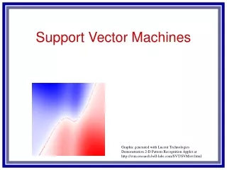
Support Vector Machines. Elegant combination of statistical learning theory and machine learning – Vapnik Good empirical results Non-trivial implementation Can be slow and memory intensive Binary classifier Much current work. SVM Comparisons.

E N D
Support Vector Machines • Elegant combination of statistical learning theory and machine learning – Vapnik • Good empirical results • Non-trivial implementation • Can be slow and memory intensive • Binary classifier • Much current work
SVM Comparisons • In order to have a natural way to compare and gain intuition on SVMs, we will first do a brief review of: • Quadric/Higher Order Machines • Radial Basis Function Networks • Note that BP follows similar strategy • Non-linear map of input features into new feature space which is now linearly separable • But, BP learns the non-linear mapping
SVM Overview • Non-linear mapping from input space into a higher dimensional feature space • Non adaptive – User defined by Kernel function • Linear decision surface (hyper-plane) sufficient in the high dimensional feature space • Note that this is the same as we do with standard MLP/BP • Avoid complexity of high dimensional feature space with kernel functions which allow computations to take place in the input space, while giving the power of being in the feature space • Get improved generalization by placing hyper-plane at the maximum margin
Standard (Primal) Perceptron Algorithm • Target minus Output not used. Just add (or subtract) a portion (multiplied by learning rate) of the current pattern to the weight vector • If weight vector starts at 0 then learning rate can just be 1 • R could also be 1 for this discussion
Dual and Primal Equivalence • Note that the final weight vector is a linear combination of the training patterns • The basic decision function (primal and dual) is • How do we obtain the coefficients αi
Dual Perceptron Training Algorithm • Assume initial 0 weight vector
Dual vs. Primal Form • Gram Matrix: all (xi·xj) pairs – Done once and stored (can be large) • αi: One for each pattern in the training set. Incremented each time it is misclassified, which would have led to a weight change in primal form • Magnitude of αi is an indicator of effect of pattern on weights (embedding strength) • Note that patterns on borders have large αiwhile easy patterns never effect the weights • Could have trained with just the subset of patterns with αi > 0 (support vectors) and ignored the others • Can train in dual. How about execution? Either way (dual can be efficient if support vectors are few) • Would if transformed feature space is still not linearly separable? αi would keep growing. Could do early stopping or bound the αi with some maximum C, thus allowing outliers.
Feature Space and Kernel Functions • Since most problems require a non-linear decision surface, we do a non-linear map Φ(x) = (Φ1(x),Φ2(x), …,ΦN(x)) from input space to feature space • Feature space can be of very high (even infinite) dimensionality • By choosing a proper kernel function/feature space, the high dimensionality can be avoided in computation but effectively used for the decision surface to solve complex problems - "Kernel Trick" • A Kernel is appropriate if the matrix of all K(xi, xj) is positive semi-definite (has non-negative eigenvalues). Even when this is not satisfied many kernels still work in practice (sigmoid).
Basic Kernel Execution Primal: Dual: • Kernel version: • Now we see the real advantage of working in the dual form • Note intuition of execution: Gaussian (and other) Kernel similar to reduced weighted K-nearest neighbor
Polynomial Kernels • For greater dimensionality can do
Polynomial Kernel Example • Assume a simple 2-d feature vector x: x1, x2 • Note that a new instance x will be paired with training vectors xi from the training set K(x, xi). We'll call these xz for this example. • Note that in the input space x we are getting the 2nd order terms: x12, x22, and x1x2
Polynomial Kernel Example • Following is the 3rd degree polynomial kernel
Polynomial Kernel Example • Note that for the 2nd degree polynomial with two variables we get the 2nd order terms x12, x22, and x1x2 • Compare with quadric. We also add bias weight with SVM. • For the 2nd degree polynomial with three variables we would get the 2nd order terms x12, x22, x32, x1x2,x1x3, and x2x3 • Note that we only get the dth degree terms. However, with some kernel creation/manipulation we could also include the lower order terms
SVM Execution • Assume novel instance x = <.4, .8> • Assume training set vectors (with bias = 0) .5, .3 y= -1 α=1 -.2, .7 y= 1 α=2 • What is the output for this case? • Show higher-order and kernel computation
Kernel Trick • So are we getting the same power as the Quadric machine without having to directly calculate the 2nd order terms?
Kernel Trick • So are we getting the same power as the Quadric machine without having to directly calculate the 2nd order terms? • No. With SVM we weight the scalar result of the kernel with constant coefficients in the 2nd order equation! • With Quadric we can have a separate learned weight (coefficient) for each term • Although do get to individually weight each support vector • Assume that the 3rd term above was really irrelevant. How would Quadric/SVM deal with that?
Kernel Trick Realities • Polynomial Kernel - all monomials of degree 2 • x1x3y1y3+ x3x3y3y3+ .... (all 2nd order terms) • K(x,y) = <Φ(x)·Φ(y)> = … + (x1x3)(y1y3) + (x3x3)(y3y3) + ... • Lot of stuff represented with just one <x·y>2 • However, in a full higher order solution we would would like adaptive coefficients for each of these higher order terms (i.e.-2x1 + 3·x1x2 + …) • SVM just sums them all with individual constant internal coefficients • Thus, not as powerful as a higher order system with arbitrary weighting • The more desirable arbitrary weighting can be done in an MLP because learning is done in the layers between inputs and hidden nodes • SVM feature to higher order feature is a fixed mapping. No learning at that level. • Of course, individual weighting requires a theoretically exponential increase in terms/hidden nodes for which we need to find weights as the polynomial degree increases. Also need learning algorithms which can actually find these most salient higher-order features.
SVM vs RBF Comparison • SVM commonly uses a Gaussian kernel • Kernel is a distance metric (ala K nearest neighbor) • How does the SVM differ from RBF?
SVM vs RBF Comparison • SVM commonly uses a Gaussian kernel • How does the SVM differ from RBF? • SVM will automatically discover which training instances to use as prototypes during the quadratic optimization • Both weight the different prototypes • RBF uses a perceptron style learning algorithm to create weights between prototypes and output classes • RBF supports multiple output classes and nodes have a vote for each output class, whereas SVM support vectors can only vote 1 or -1 • SVM will create a maximum margin decision surface based on the chosen weighted support vectors • Since internal feature coefficients are constants in the Gaussian distance kernel (for both SVM and RBF), SVM will suffer from fixed/irrelevant features just like RBF • Same Kernel Trick weakness – no learning in the kernel map from input to higher order feature space
Choosing a Kernel • Can start from a desired feature space and try to construct kernel • More often one starts from a reasonable kernel and may not analyze the feature space • Some kernels are a better fit for certain problems, domain knowledge can be helpful • Common kernels: • Polynomial • Gaussian • Sigmoidal • Application specific
Maximum Margin • Maximum margin can lead to overfit due to noise • Problem may not be linearly separable even in transformed feature space • Soft Margin is a common solution, allows slack variables • αi constrained to be >= 0 and less than C. The C allows outliers. • How to pick C? Can try different values for the particular application to see which works best.
Quadratic Optimization • Optimizing the margin in the higher order feature space is convex and thus there is one guaranteed solution at the minimum (or maximum) • SVM Optimizes the dual representation (avoiding the higher order feature space) • Maximizing Σαi tends towards larger α subject to Σαiyi= 0 and α≤ C (tends towards smaller α) • Without this term, α = 0 would suffice • 2nd term minimizes number of support vectors since • Two positive (or negative) instances that are similar (high Kernel result) would increase size of term. Note that both (or either) instances usually not needed. • Two non-matched instances which are similar should have larger α since they are likely support vectors at the decision boundary (negative term helps maximize) • The optimization is quadratic in the αi terms and linear in the constraints – can drop C maximum for non soft margin • While quite solvable, requires complex code and usually done with a numerical methods software package – Quadratic programming
Execution • Typically use dual form which can take advantage of Kernel efficiency • If the number of support vectors is small then dual is fast • In cases of low dimensional feature spaces, could derive weights from αi and use normal primal execution • Approximations to dual are possible to obtain speedup (smaller set of prototypical support vectors)
Standard SVM Approach • Select a 2 class training set, a kernel function (calculate the Gram Matrix), and choose the Cvalue (soft margin parameter) • Pass these to a Quadratic optimization package which will return an α for each training pattern based on the following (non-bias version) • Patterns with non-zero α are the support vectors for the maximum margin SVM classifier. • Execute by using the support vectors
A Simple On-Line Alternative • Stochastic on-line gradient ascent • Can be effective • This version assumes no bias • Sensitive to learning rate • Stopping criteria tests whether it is an appropriate solution – can just go until little change is occurring or can test optimization conditions directly • Can be quite slow and usually quadratic programming is used to get an exact solution • Newton and conjugate gradient techniques also used – Can work well since it is a guaranteed convex surface – bowl shaped
Maintains a margin of 1 (typical in standard SVM implementation) which can always be done by scaling or equivalently w and b • This is done with the (1-actual) term below, which can update even when correct, as it tries to make the distance of support vectorss tothe decision surface be exactly 1
Large Training Sets • Big problem since the Gram matrix (all (xi·xj) pairs) is O(n2) for n data patterns • 106 data patterns require 1012 memory items • Can’t keep them in memory • Also makes for a huge inner loop in dual training • Key insight: most of the data patterns will not be support vectors so they are not needed
Chunking • Start with a reasonably sized subset of the Data set (one that fits in memory and does not take too long during training) • Train on this subset and just keep the support vectors or the m patterns with the highest αi values • Grab another subset, add the current support vectors to it and continue training • Note that this training may allow previous support vectors to be dropped as better ones are discovered • Repeat until all data is used and no new support vectors are added or some other stopping criteria is fulfilled
SVM Issues • Excellent empirical and theoretical potential • Multi-class problems not handled naturally. Basic model classifies into just two classes. Can do one model for each class (class i is 1 and all else 0) and then decide between conflicting models using confidence, etc. • How to choose kernel – main learning parameter other than margin penalty C. Kernel choice will include other parameters to be defined (degree of polynomials, variance of Gaussians, etc.) • Speed and Size: both training and testing, how to handle very large training sets (millions of patterns and/or support vectors) not yet solved • Adaptive Kernels: trained during learning?