Download
1 / 32
320 likes | 325 Views
Quantifying Chaos. Introduction Time Series of Dynamical Variables Lyapunov Exponents Universal Scaling of the Lyapunov Exponents Invariant Measures Kolmogorov-Sinai Entropy Fractal Dimensions Correlation Dimension & a Computational History Comments & Conclusions. 1. Introduction.

E N D
Quantifying Chaos • Introduction • Time Series of Dynamical Variables • Lyapunov Exponents • Universal Scaling of the Lyapunov Exponents • Invariant Measures • Kolmogorov-Sinai Entropy • Fractal Dimensions • Correlation Dimension & a Computational History • Comments & Conclusions
1. Introduction Why quantify chaos? • To distinguish chaos from noise / complexities. • To determine active degrees of freedom. • To discover universality classes. • To relate chaotic parameters to physical quantities.
2. Time Series of Dynamical Variables • (Discrete) time series data: • x(t0), x(t1), …, x(tn) • Time-sampled (stroboscopic) measurements • Poincare section values • Real measurements & calculations are always discrete. • Time series of 1 variable of n-D system : • If properly chosen, essential features of system can be re-constructed: • Bifurcations • Chaos on-set • Choice of sampling interval is crucial if noise is present (see Chap 10) • Quantification of chaos: • Dynamical: • Lyapunov exponents • Kolmogorov-Sinai (K-S) Entropy • Geometrical: • Fractal dimension • Correlation dimension • Only 1-D dissipative systems are discussed in this chapter.
9.3. Lyapunov Exponents Time series: Given i & j, let System is chaotic if with Lyapunov exponent • Technical Details: • Check exponential dependence. • λ is x dependent → λ = Σiλ(xi) / N . • N can’t be too large for bounded systems. • λ = 0 for periodic system. • i & j shouldn’t be too close. • Bit- version: dn = d02nλ Logistic Map
9.4. Universal Scaling of the Lyapunov Exponents Period-doubling route to chaos: Logistic map: A = 3.5699… LyapunovExponents.nb λ < 0 in periodic regime. λ = 0 at bifurcation point. (period-doubling) λ > 0 in chaotic regime. λ tends to increase with A → More chaotic as A increases.
Huberman & Rudnick: λ(A > A) is universal for periodic-doubling systems: = Feigenbaum δ λ~ order parameter AA ~ T TC λ0 = 0.9
Derivation of the Universal Law for λ Logistic map • Chaotic bands merge via “period-undoubling” for A > A. • Ratio of convergence tends to Feigenbaum δ.
Let 2m bands merge to 2m1 bands at A = Am . • Reminder: 2m bands bifurcate to 2m+1 bands at A = Am . Divergence of trajectories in 1 band : Divergence of trajectories among 2m band : λ = effective Lyapunov exponent denoting 2m iterations as one. λ = Lyapunov exponent for If λ is the same for all bands, then Ex.2.4-1: Assuming δn = δ gives Similarly:
→ → i.e.,
9.5. Invariant Measures For systems of large DoFs, geometric analysis becomes unwieldy. Alternative approach: Statistical methods. Basic quantity of interest: Probability of trajectory to pass through given region of state space. • Definition of Probability • Invariant Measures • Ergodic Behavior
Definition of Probability Consider an experiment with N possible results (outcomes). After M runs (trials) of the experiment, let there be mi occurrences of the ith outcome. The probabilitypi of the ith outcome is defined as where → ( Normalization ) If the outcomes are described by a set of continuous parameters x, N = . mi are finite → M= and pi= 0 i. Remedy: Divide range of x into cells/bins. mi = number of outcomes belonging to the ith cell.
Invariant Measures • For an attractor in state space: • Divide attractor into cells. • 1-D case: pi mi / M. • Set {pi} is a natural probability measure if it is independent of (almost all) IC. = probability of trajectory visiting cell i. p(x) dx = probability of trajectory visiting interval [ x, x+dx ] or [ xdx/2, x+dx/2 ]. Let then μ is an invariant probability measure if Treating M as total mass → p(x) = ρ(x)
Example: Logistic Map, A = 4 From § 4.8: For A = 4, logistic map is equivalent to Bernoulli shift. with → → → Numerical: 1024 iterations into 20 bins
Ergodic Behavior Time average of B(x): Bt should be independent of t0 as T → . Ensemble average of B(x): • Comments: • Bp is meaningful only for invariant probability measures. • p(x) may not exist, e.g., strange attractors. System is ergodic if Bt = Bp .
Example: Logistic Map, A = 4 Local values of the Lyapunov exponent: Ensemble average value of the Lyapunov exponent: ( same as the Bernoulli shift ) Same as that calculated by time average (c.f. §5.4):
9.6. Kolmogorov-Sinai Entropy • Brief Review of Entropy: • Microcanonical ensemble (closed, isolated system in thermal equilibrium): • S = k ln N = k ln pp = 1/N • Canonical ensemble (small closed subsystem): • S = k Σipi ln pi Σipi = 1 • 2nd law: ΔS 0 for spontaneous processes in closed isolated system. • → S is maximum at thermodynamic equilibrium • Issue: No natural way to count states in classical mechanics. • → S is defined only up to an constant ( only ΔS physically meaningful ) • Quantum mechanics: phase space volume of each state = hn , n = DoF.
Entropy for State Space Dynamics • Divide state space into cells (e.g., hypercubes of volume LDof ). • For dissipative systems, replace state space with attractors. • Start evolution for an ensemble of I.C.s (usually all located in 1 cell). • After n time steps, count number of states in each cell. k = Boltzmann constant Note: • Non-chaotic motion: • Number of cells visited (& hence S) is independent of t & M on the macroscopic time-scale. • Chaotic motion: • Number of cells visited (& hence S)increases with t but independent of M. • Random motion: • Number of cells visited (& hence S ) increases with both t & M
Only ΔS is physically significant. Kolmogorov-Sinai entropy rate = K-S entropy = K is defined as For iterated maps or Poincare sections, τ= 1 so that E.g., if the number of occupied cells Nn is given by and all occupied cells have the same probability then Pesin identity: λi = positive average Lyapunov exponents
Alternative Definition of the K-S Entropy See Schuster • Map out attractor by running a single trajectory for a long time. • Divide attractor into cells. • Start a trajectory of N steps & mark the cell it’s in at t = nτas b(n). • Do the same for a series of other slightly different trajectories starting from the same initial cell. • Calculate the fraction p(i) of trajectories described by the ith cell sequence. Then where Exercise: Show that both definitions of K give roughly the same result for all 3 types of motions discussed earlier.
9.7. Fractal Dimensions Geometric aspects of attractors Distribution of state space points of a long time series → Dimension of attractor • Importance of dimensionality: • Determines range of possible dynamical behavior. • Dictates long-term dynamics. • Reveals active degrees of freedom. • For a dissipative system : • D < d, • D dimension of attractor, • d dimension of state space. • D* < D, • D* = dimension of attractor on Poincare section.
For a Hamiltonian system, • D d 1, • D = dimension of points generated by one trajectory • ( trajectory is confined on constant energy surface ) • D* < D, • D* = dimension of points on Poincare section. • Dimension is further reduced if there are other constants of motion. Example: 3-D state space → attractor must shrink to a point or a curve → system can’t be quasi-periodic ( no torus ) → no q.p. solutions for the Lorenz system. Dissipative system: Strange attractor = Attractor with fractional dimensions (fractals) Caution: There’re many inequivalent definitions of fractal dimension. See J.D.Farmer, E.Ott, J.A.Yorke, Physica D7, 153-80 (1983)
Capacity ( Box-Counting ) Dimension Db • Easy to understand. • Not good for high d systems. 1st used by Komogorov N(R) = Number of boxes of side R that covers the object
Example 1: Points in 2-D space A single point: Box = square of sides R. → Set of N isolated points: Box = square of sides R. R = ½ (minimal distance between points). → Example 2: Line segment of length L in 2-D space Box = square of sides R. →
Example 3: Cantor Set Starting with a line segment of length 1, take out repeatedly the middle third of each remaining segment. Caution: Given M finite, set consists of 2M line segments → Db = 1. Given M infinite, set consists of discrete points → Db = 0. Limits M → and R → 0 must be taken simultaneously. At step M, there remain 2M segments, each of length 1/3M.
Measure of the Cantor set: Length of set Ex. 9.7-5: Fat Fractal
Example 4: Koch Curve Start with a line segment of length 1. a) Construct an equilateral triangle with the middle third segment as base. b) Discard base segment. Repeat a) and b) for each remaining segment. At step M, there exists 4M segments of length 1/3M each.
Types of Fractals • Fractals with self-similarity: • small section of object, when magnified, is identical with the whole. • Fractals with self-affinity: • same as self-similarity, but with anisotropic magnification. • Deterministic fractals: • Fixed construction rules. • Random fractals: • Stochastic construction rules (see Chap 11).
Fractal Dimensions of State Space Attractors Difficulty: R → 0 not achievable due to finite precision of data. Remedy: Alternate definition of fractal dimension (see §9.8) Logistic map at A, renormalization method: Db= 0.5388… (universal) Elementary estimates: Consider A → A+( from above ). Sarkovskii’s theorem → chaotic bands undergo doubling-splits as A → A+. Feigenbaum universality → splitted bands are narrower by 1/α and 1/α2 . Assume points in each band distributed uniformly → splitting is Cantor-set like.
1st estimate: R decreases by factor 1/α at each splitting. → 2nd estimate: → Dbprocedure dependent. An infinity of dimensional measures needed to characterize object (see Chap 10)