Download
1 / 23
230 likes | 350 Views
HST Key Project on the Extragalactic Distance Scale. Presentation by Alaine Ginocchio May 5, 2006. HST Key Project. Measuring an accurate value of H 0 was one of the motivating reasons for building NASA/ESA Hubble Space Telescope (HST).

E N D
HST Key Project on the Extragalactic Distance Scale Presentation by Alaine Ginocchio May 5, 2006
HST Key Project • Measuring an accurate value of H0 was one of the motivating reasons for building NASA/ESA Hubble Space Telescope (HST). • Measurement of H0 with the goal of 10% accuracy was designated as one of the three “Key Projects” of the HST –Mid 1980’s
Measuring H0 • Overall Goal: measure H0 based on a Cepheid calibration of a number of independent, secondary distance determination methods • Locate Cepheids, measure distances to galaxies, calibrate secondary methods: • Tulley-Fisher relation • Type Ia supernovae • the fundamental plane for elliptical galaxies • surface brightness fluctuations • Type II supernovae
Outline • The status of H0 prior to HST • Using Cepheid variable stars to measure distances • Secondary Methods • The Key Project • Results
The Hubble Constant • 1929 Edwin Hubble publishes results: correlation between the distances to galaxies and their recession velocities v=H0d (evidence that the universe is expanding) • It has been over 7 decades trying to pin down accurate H0, primary difficulty establishing accurate distances over cosmologically significant scales
Prior to HST • Arguing over H0 by factor of 2 (50-100km s-1 Mpc-1) • Atmospheric seeing set limit for resolving Cepheids to only a few Mpc’s, confined to search Local Group of galaxies and very nearest surrounding groups: • 5 galaxies with well-measured Cepheids provided absolute calibration for Tully-Fisher relation • A single Cepheid distance provided calibration for surface brightness fluctuation method • No Cepheid calibrators for Type Ia Supernovae • HST extends seeing limit 10 fold (vol thousand fold)
Cepheid Variable Stars • 1907, Henrietta Leavitt (1868-1921), Harvard Observatory Astronomer, discovers CV’s luminosity and period follow very tight correlation • Longer period = brighter CV
Why Cepheids Pulsate • Vary in luminosity because they actually pulsate in and out in size (get brighter as they grow larger, dim as they shrink) • Can’t achieve balance of power welling up from core and power radiating from surface • Upper layers of star too opaque, pressure blds beneath photosphere, star expands in size • Outer layer puffs, becomes more transparent, energy escapes, underlying pressure drops, star contracts • Larger and more luminous CVs take longer to pulsate in and out , period ranges from 2-150 days • Light curve with saw tooth signature P~50 days Type I: heavy element content similar to sun
Cepheid Variables • Det luminosity to within ~10% • Most important primary distance indicator for nearby galaxies • 2 populations of CVs (Hubble’s mistake ) • Type one: classical type, ~4 times brighter than type 2, have a high metallicity, found in disk. • Type two: older stars, low metallicity, found in halo • Reach is limited to ~ 30Mpc • But you can use it to calibrate secondary methods to extend reach
Secondary MethodsTully-Fisher Relation • Most commonly applied distance indicator (2001) • Relationship between total luminosity spiral galaxy and rotation speed of disk • Faster rotation=more luminous • L~V4 scaling law appears to be a general property of galaxies • Scatter +-0.3mag or +- 15% distance for a single galaxy • Total (corrected to face on) luminosity is strongly correlated with the max rotation velocity of galaxy (corrected to edge-on inclination) • Flat rotation curves of spirals which produce well defined circular velocities • Find speed from Doppler shift, tells you L, makes galaxy a standard candle
Secondary Method: Ia Supernovae • White dwarf supernovae, exploding white dwarf stars that have reached the 1.4 solar mass white dwarf limit • Should have same luminosity because come from stars of same mass that explode in same way • Determine true luminosity by using CVs to measure distance to galaxies • Confirm L of all WD SNs are about the same • BRIGHT: 10 bill solar luminosities at peak, detect ~ 10 bill lt-yrs away • But, occur only once every few hundred years and need to catch within 1-2 days of explosion White dwarf supernovae in galaxies approx 10 billion lt yrs away. Upper image shows what galaxies look like without supernovae . HST Images
Supernova 1994D in Galaxy NGC 4526, May 25, 1999, HST Key Project
Secondary Methods • Fundamental plane for elliptical galaxies • EG: correlation between the stellar velocity dispersion and the intrinsic luminosity • EGs found to occupy a “fundamental plane” in which a defined effective radius is tightly correlated with the surface brightness with that radius and central velocity dispersion • Scatter ~10-20% distance for individual cluster • surface brightness fluctuations • The resolution of stars in galaxies is distance dependent • Elliptical or spirals with prominent bulges • Normalizing to the mean total flux and correcting for an observed color dependence, relative distances to galaxies can be measured • Intrinsic scatter factor of 3 improvement to T-F or F-Plane • Type II supernovae • Supernova from massive stars, fainter and show wider variation in luminosity than IaSN • Baade-Wesselink technique: follow spectral fits of color T, flux and radial vel of envelope over time to det dist. • Applied independent of local calibration of extragalactic distance scale but verified with galaxies of known distances & diversity of methods constrains overall systematic errors
Key Project • 1984 Conceptually Begins • 1991 First Observations • 1998 Last observations finished • 2001 Final results published • Main goal: determine H0 to an accuracy of 10% by: (1) refining the cosmic distance scale by observing 18 spiral galaxies within 20 Mpc, searching for and measuring the periods and magnitudes of Cepheid variables (2) calibrating the secondary distance indicators (3) Measure H0 with secondary distance indicators and combine
Total Cepheid Calibration Sample • 18 galaxies: Key Project • 8 galaxies: reanalyzed HST archival data observed by other groups • 5 very nearby galaxies • 31 Galaxies: subsets used to calibrate secondary models • Discovered 800 CVs in 18 galaxies out to 65 million lt yrs. • CV positions magnitudes and periods available on http://www.ipac.caltech.edu/H0kp/H0KeyProj.html
Among brightest stellar indicators, relatively young stars, found in abundance in spiral galaxies Many independent objects can be observed in a single galaxy Large amplitude & distinct sawtooth light curve facilitate discovery Long lifetimes: can be observed at other times and wavelengths CV P-L relationship has small scatter (I-band dispersion ~+-0.1 mag) Have been studied and theoretically modeled extensively and their physics is understood Young stars so found in regions with dust scattering, absorption and reddening. Corrections must be made for extinction with assumptions Metallicity: dependence of PL relationship on chemical composition very difficult to quantify (PL relationship has slight dependence on metallicity) Accurate calibration of PL relation at any given metallicity not yet established Crowding effects Limited reach ~30 Mpc Strengths and Weaknesses of CV s
Methodology • Combine values of H0 from different secondary methods • All based on a common Cepheid 0-point but with different subsets of Cepheid calibrators • Take out peculiar velocity • Used 3 methods: classical frequentist analysis, Bayesian analysis and weighting scheme based on numerical simulations • All in good agreement • Conclusion: combined value is robust, the choice of statistical method not determine result
Uncertainties in H0 for Secondary Methods Error Method H0 (random, systematic) Refs (%) 36 Type Ia SN, 4000\cz\30,000 km s~1 . . . . . . 71 2 6 1, 2, 3, 4 21 TF clusters, 1000\cz\9000 km s~1 . . . . . .. . 71 3 7 5, 6, 7 11 FP clusters, 1000\cz\11,000 km s~1 . . .... . 82 6 9 8, 9 SBF for 6 clusters, 3800\cz\5800 km s~1 . . ... . 70 5 6 10, 11 4 Type II SN, 1900\cz\14,200 km s~1 . . . . . .. . 72 9 7 12 “\” = “<“ NOTE: Combined values of (random) km s~1 Mpc~1 (Bayesian), H0: H0\722 H0\723 (random) km s~1 Mpc~1 (frequentist) ; (random) km s~1 Mpc~1 (Monte Carlo) H0\723 REFERENCES.È(1) Hamuy et al. 1996; (2) Riess et al. 1998; (3) Jha et al. 1999; (4) Gibson et al. 2000a; (5) Giovanelli et al. 1997; (6) Aaronson et al. 1982, 1986; (7) Sakai et al. 2000; (8) Jorgensen et al. 1996; (9) Kelson et al. 2000; (10) Lauer et al. 1998; (11) Ferrarese et al. 2000a; (12) Schmidt et al. 1994.
Hubble diagram of distance vs. velocity for secondary distance indicators calibrated by CVs. Velocities are corrected for the nearby flow model of Mould et al. (2000). A slope of H0=72 is shown, flanked by +-10% lines. Beyond 5000 km s-1 (vertical line), both numerical simulations and observations suggest that the effects of peculiar motions are small.
Combined RESULT FOR H0 H0=72 +-8 km s-1 Mpc-1