Download
1 / 7
70 likes | 191 Views
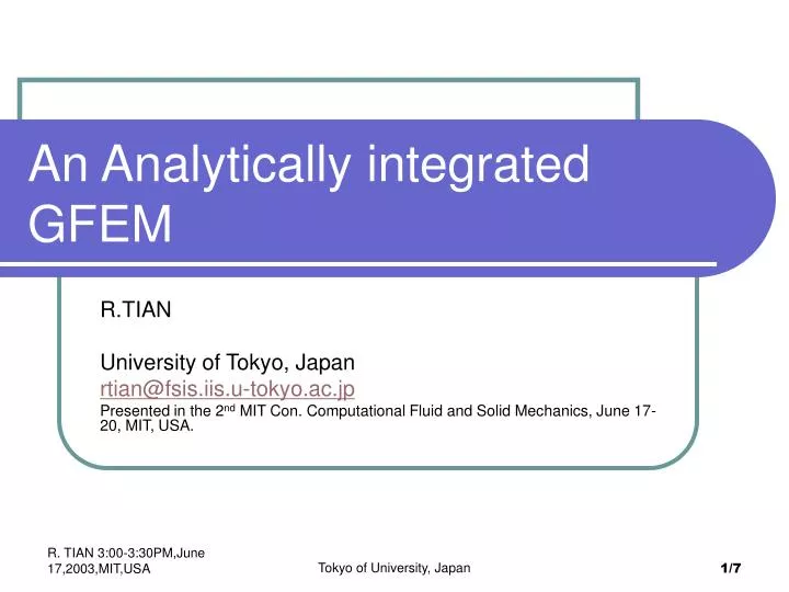
An Analytically integrated GFEM. R.TIAN University of Tokyo, Japan rtian@fsis.iis.u-tokyo.ac.jp Presented in the 2 nd MIT Con. Computational Fluid and Solid Mechanics, June 17-20, MIT, USA. Motivation. The GFEM approximations compared with FEMs’

E N D
An Analytically integrated GFEM R.TIAN University of Tokyo, Japan rtian@fsis.iis.u-tokyo.ac.jp Presented in the 2nd MIT Con. Computational Fluid and Solid Mechanics, June 17-20, MIT, USA. Tokyo of University, Japan
Motivation • The GFEM approximations compared with FEMs’ • Local approximations can be custom tailored to the problem under consideration. • Polynomials are mostly used in constructing the local approximations. • Adaptive quadratures or quadrature rules using many evaluation points have to be employed for high order of polynomials, which cost lots of CPU time. • An analytical approach, if exists, should be necessary.
Element e Possible FE meshes • A triangular or rectangular element with simple shape function is generated independently of the boundary of the domain. • The regular FE meshes are be suitable for any problems with geometrically complex boundaries. • The use of the simple FE meshes results in irregular and even concave elements, on which further subdivision for quadratures has to be performed. • An analytical integration saves not only effort for the element subdivision but also CPU time of the quadratures.
Consider an element with n counter-clockwise ordered vertex P1,P2,…,Pn. K1+k2 ranging from 0 to12 are formulated. y P1 Pn P2 e Pi P3 P0 x Analytical Integration on a Simplex The integration also applies in 3 dimensions.
10 15 A 2 B 15 Example: Computational effort comparison • Model: • GFEM meshes: (T3:Triangular FE and R4: Rectangular FE) T3 T3 R4 Load flag Fixed points Independent FE meshes
Deformation by only one GFE and Computational efforts Deformed configuration of both the FE mesh and the beam. See the right figure for the computational effort comparison between numerical integrations and the analytical integration. It is clear that the numerical integration costs much more CPU time as the higher order polynomials used.
Concluding Remarks • Because FE meshes can be generated independently of the domain of interest, these simple FEs like T3 and R4 are always available, specially for domains with geometrically complex boundaries. Therefore, the analytical integration proposed here is of general use. • Quadratures need much more evolution points as the order of polynomials increased and cost much more CPU time. The analytical integration then can save lots of CPU time compared to the numerical quadrature. • References (omitted.) The End. Thank you.