Download
1 / 159
1.59k likes | 1.71k Views
Performance Understanding, Prediction, and Tuning at the Berkeley Institute for Performance Studies (BIPS). Katherine Yelick Lawrence Berkeley National Laboratory and U. C. Berkeley, EECS Dept. November 2004. Outline. Motivation for Automatic Performance Tuning

E N D
Performance Understanding, Prediction, and Tuning at the Berkeley Institute for Performance Studies (BIPS) Katherine Yelick Lawrence Berkeley National Laboratory and U. C. Berkeley, EECS Dept. November 2004
Outline • Motivation for Automatic Performance Tuning • Recent results for sparse matrix kernels • Application to T3P, Omega3P • OSKI = Optimized Sparse Kernel Interface • Future Work
Prizes • Best Paper, Intern. Conf. Parallel Processing, 2004 • “Performance models for evaluation and automatic performance tuning of symmetric sparse matrix-vector multiply” • Best Student Paper, Intern. Conf. Supercomputing, Workshop on Performance Optimization via High-Level Languages and Libraries,2003 • Best Student Presentation too, to Richard Vuduc • “Automatic performance tuning and analysis of sparse triangular solve” • Finalist, Best Student Paper, Supercomputing 2002 • To Richard Vuduc • “Performance Optimization and Bounds for Sparse Matrix-vector Multiply” • Best Presentation Prize, MICRO-33: 3rd ACM Workshop on Feedback-Directed Dynamic Optimization, 2000 • To Richard Vuduc • “Statistical Modeling of Feedback Data in an Automatic Tuning System”
Motivation for Automatic Performance Tuning • Historical trends • Sparse matrix-vector multiply (SpMV): 10% of peak or less • 2x faster than CSR with “hand-tuning” • Tuning becoming more difficult over time • Performance depends on machine, kernel, matrix • Matrix known at run-time • Best data structure + implementation can be surprising • Our approach: empirical modeling and search • Up to 4x speedups and 31% of peak for SpMV • Many optimization techniques for SpMV • Several other kernels: triangular solve, ATA*x, Ak*x • Proof-of-concept: Integrate with Omega3P • Release OSKI Library, integrate into PETSc
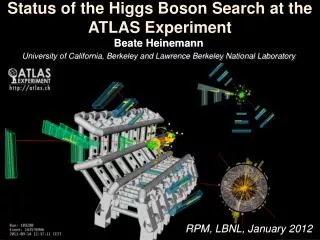
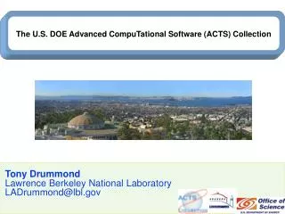
Example: The Difficulty of Tuning • n = 21216 • nnz = 1.5 M • kernel: SpMV • Source: NASA structural analysis problem • 8x8 dense substructure
Best: 4x2 Reference Speedups on Itanium 2: The Need for Search Mflop/s Mflop/s
Ultra 2i - 9% 63 Mflop/s Ultra 3 - 6% 109 Mflop/s SpMV Performance (Matrix #2): Generation 2 35 Mflop/s 53 Mflop/s Pentium III - 19% Pentium III-M - 15% 96 Mflop/s 120 Mflop/s 42 Mflop/s 58 Mflop/s
Power3 - 13% 195 Mflop/s Power4 - 14% 703 Mflop/s SpMV Performance (Matrix #2): Generation 1 100 Mflop/s 469 Mflop/s Itanium 1 - 7% Itanium 2 - 31% 225 Mflop/s 1.1 Gflop/s 103 Mflop/s 276 Mflop/s
Extra Work Can Improve Efficiency! • More complicated non-zero structure in general • Example: 3x3 blocking • Logical grid of 3x3 cells • Fill-in explicit zeros • Unroll 3x3 block multiplies • “Fill ratio” = 1.5 • On Pentium III: 1.5x speedup!
Summary of Performance Optimizations • Optimizations for SpMV • Register blocking (RB): up to 4x over CSR • Variable block splitting: 2.1x over CSR, 1.8x over RB • Diagonals: 2x over CSR • Reordering to create dense structure + splitting: 2x over CSR • Symmetry: 2.8x over CSR, 2.6x over RB • Cache blocking: 2.2x over CSR • Multiple vectors (SpMM): 7x over CSR • And combinations… • Sparse triangular solve • Hybrid sparse/dense data structure: 1.8x over CSR • Higher-level kernels • AAT*x, ATA*x: 4x over CSR, 1.8x over RB • A2*x: 2x over CSR, 1.5x over RB
Potential Impact on Applications: T3P • Source: SLAC [Ko] • 80% of time spent in SpMV • Relevant optimization techniques • Symmetric storage • Register blocking • On Single Processor Itanium 2 • 1.68x speedup • 532 Mflops, or 15% of 3.6 GFlop peak • 4.4x speedup with 8 multiple vectors • 1380 Mflops, or 38% of peak
Potential Impact on Applications: Omega3P • Application: accelerator cavity design [Ko] • Relevant optimization techniques • Symmetric storage • Register blocking • Reordering • Reverse Cuthill-McKee ordering to reduce bandwidth • Traveling Salesman Problem-based ordering to create blocks • Nodes = columns of A • Weights(u, v) = no. of nz u, v have in common • Tour = ordering of columns • Choose maximum weight tour • See [Pinar & Heath ’97] • 2x speedup on Itanium 2, but SPMV not dominant
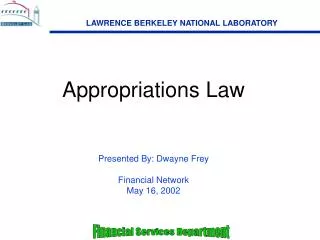
“Microscopic” Effect of RCM Reordering Before: Green + Red After: Green + Blue
“Microscopic” Effect of Combined RCM+TSP Reordering Before: Green + Red After: Green + Blue
Optimized Sparse Kernel Interface - OSKI • Provides sparse kernels automatically tuned for user’s matrix & machine • BLAS-style functionality: SpMV.,TrSV, … • Hides complexity of run-time tuning • Includes new, faster locality-aware kernels: ATA*x, … • Faster than standard implementations • Up to 4x faster matvec, 1.8x trisolve, 4x ATA*x • For “advanced” users & solver library writers • Available as stand-alone library (Oct ’04) • Available as PETSc extension (Dec ’04) • Lines of code: ?? written by us, ?? generated
How the OSKI Tunes (Overview) Application Run-Time Library Install-Time (offline) 1. Build for Target Arch. 2. Benchmark Workload from program monitoring History Matrix Generated code variants Benchmark data 1. Evaluate Models Heuristic models 2. Select Data Struct. & Code To user: Matrix handle for kernel calls Extensibility: Advanced users may write & dynamically add “Code variants” and “Heuristic models” to system.
How the OSKI Tunes (Overview) • At library build/install-time • Pre-generate and compile code variants into dynamic libraries • Collect benchmark data • Measures and records speed of possible sparse data structure and code variants on target architecture • Installation process uses standard, portable GNU AutoTools • At run-time • Library “tunes” using heuristic models • Models analyze user’s matrix & benchmark data to choose optimized data structure and code • Non-trivial tuning cost: up to ~40 mat-vecs • Library limits the time it spends tuning based on estimated workload • provided by user or inferred by library • User may reduce cost by save tuning results for application on future runs with same or similar matrix
Optimizations in the Initial OSKI Release • Fully automatic heuristics for • Sparse matrix-vector multiply • Register-level blocking • Register-level blocking + symmetry + multiple vectors • Cache-level blocking • Sparse triangular solve with register-level blocking and “switch-to-dense” optimization • Sparse ATA*x with register-level blocking • User may select other optimizations manually • Diagonal storage optimizations, reordering, splitting; tiled matrix powers kernel (Ak*x) • All available in dynamic libraries • Accessible via high-level embedded script language • “Plug-in” extensibility • Very advanced users may write their own heuristics, create new data structures/code variants and dynamically add them to the system
Example: Combining Optimizations • Register blocking, symmetry, multiple (k) vectors • Three low-level tuning parameters: r, c, v X k v * r c += Y A
Example: Combining Optimizations • Register blocking, symmetry, and multiple vectors [Ben Lee @ UCB] • Symmetric, blocked, 1 vector • Up to 2.6x over nonsymmetric, blocked, 1 vector • Symmetric, blocked, k vectors • Up to 2.1x over nonsymmetric, blocked, k vecs. • Up to 7.3x over nonsymmetric, nonblocked, 1, vector • Symmetric Storage: 64.7% savings
Current Work • Public software release • Impact on library designs: Sparse BLAS, Trilinos, PETSc, … • Integration in large-scale applications • DOE: Accelerator design; plasma physics • Geophysical simulation based on Block Lanczos (ATA*X; LBL) • Systematic heuristics for data structure selection? • Evaluation of emerging architectures • Revisiting vector micros • Other sparse kernels • Matrix triple products, Ak*x • Parallelism • Sparse benchmarks (with UTK) [Gahvari & Hoemmen] • Automatic tuning of MPI collective ops [Nishtala, et al.]
Review of Tuning by Illustration (Extra Slides)
Splitting for Variable Blocks and Diagonals • Decompose A = A1 + A2 + … At • Detect “canonical” structures (sampling) • Split • Tune each Ai • Improve performance and save storage • New data structures • Unaligned block CSR • Relax alignment in rows & columns • Row-segmented diagonals
Example: Variable Block Row (Matrix #12) 2.1x over CSR 1.8x over RB
Example: Row-Segmented Diagonals 2x over CSR
Raefsky4 (structural problem) + SuperLU + colmmd N=19779, nnz=12.6 M Dense trailing triangle: dim=2268, 20% of total nz Can be as high as 90+%! 1.8x over CSR Example: Sparse Triangular Factor
“axpy” dot product Cache Optimizations for AAT*x • Cache-level: Interleave multiplication by A, AT • Register-level: aiT to be r´c block row, or diag row • Algorithmic-level transformations for A2*x, A3*x, …
Summary • Automated block size selection • Empirical modeling and search • Register blocking for SpMV, triangular solve, ATA*x • Not fully automated • Given a matrix, select splittings and transformations • Lots of combinatorial problems • TSP reordering to create dense blocks (Pinar ’97; Moon, et al. ’04)
A Sparse Matrix You Encounter Every Day Who am I? I am a Big Repository Of useful And useless Facts alike. Who am I? (Hint: Not your e-mail inbox.)
Problem Context • Sparse kernels abound • Models of buildings, cars, bridges, economies, … • Google PageRank algorithm • Historical trends • Sparse matrix-vector multiply (SpMV): 10% of peak • 2x faster with “hand-tuning” • Tuning becoming more difficult over time • Promise of automatic tuning: PHiPAC/ATLAS, FFTW, … • Challenges to high-performance • Not dense linear algebra! • Complex data structures: indirect, irregular memory access • Performance depends strongly on run-time inputs
Key Questions, Ideas, Conclusions • How to tune basic sparse kernels automatically? • Empirical modeling and search • Up to 4x speedups for SpMV • 1.8x for triangular solve • 4x for ATA*x; 2x for A2*x • 7x for multiple vectors • What are the fundamental limits on performance? • Kernel-, machine-, and matrix-specific upper bounds • Achieve 75% or more for SpMV, limiting low-level tuning • Consequences for architecture? • General techniques for empirical search-based tuning? • Statistical models of performance
Road Map • Sparse matrix-vector multiply (SpMV) in a nutshell • Historical trends and the need for search • Automatic tuning techniques • Upper bounds on performance • Statistical models of performance
Compressed Sparse Row (CSR) Storage Matrix-vector multiply kernel: y(i) y(i) + A(i,j)*x(j) Matrix-vector multiply kernel: y(i) y(i) + A(i,j)*x(j) for each row i for k=ptr[i] to ptr[i+1] do y[i] = y[i] + val[k]*x[ind[k]] Matrix-vector multiply kernel: y(i) y(i) + A(i,j)*x(j) for each row i for k=ptr[i] to ptr[i+1] do y[i] = y[i] + val[k]*x[ind[k]]
Road Map • Sparse matrix-vector multiply (SpMV) in a nutshell • Historical trends and the need for search • Automatic tuning techniques • Upper bounds on performance • Statistical models of performance
Historical Trends in SpMV Performance • The Data • Uniprocessor SpMV performance since 1987 • “Untuned” and “Tuned” implementations • Cache-based superscalar micros; some vectors • LINPACK
Example: The Difficulty of Tuning • n = 21216 • nnz = 1.5 M • kernel: SpMV • Source: NASA structural analysis problem
Still More Surprises • More complicated non-zero structure in general
Still More Surprises • More complicated non-zero structure in general • Example: 3x3 blocking • Logical grid of 3x3 cells
Historical Trends: Mixed News • Observations • Good news: Moore’s law like behavior • Bad news: “Untuned” is 10% peak or less, worsening • Good news: “Tuned” roughly 2x better today, and improving • Bad news: Tuning is complex • (Not really news: SpMV is not LINPACK) • Questions • Application: Automatic tuning? • Architect: What machines are good for SpMV?
Road Map • Sparse matrix-vector multiply (SpMV) in a nutshell • Historical trends and the need for search • Automatic tuning techniques • SpMV [SC’02; IJHPCA ’04b] • Sparse triangular solve (SpTS) [ICS/POHLL ’02] • ATA*x [ICCS/WoPLA ’03] • Upper bounds on performance • Statistical models of performance