PRINCIPAL COMPONENT ANALYSIS OF VARIABLE STAR LIGHT CURVES

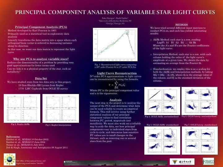
1. PRINCIPAL COMPONENT ANALYSIS OF VARIABLE STAR LIGHT CURVES Ruka Murugan1, Shashi Kanbur2 1University of Rochester, Rochester, NY 2Oswego, Oswego, NY • METHODS • We have tried several different input matrices to conduct PCA on, and each has yielded interesting results: • AkBk Method: each star is a row, reading: • Log(P) A1 B1 A2 B2 … AkBk • Where the A’s and B’s are the Fourier coefficients • of the light curve. • Interpolation Method: each star is a row, with each column holding the value of the light curve’s amplitude at a given time. We obtain the data by estimating an average from the Fourier fit. • Standardization: we employ this is as a scaling for both the AkBk and Interpolation methods, by taking Mij= (Mij – Aj )/Sj, where Aj is the average value of the column, and Sj is the standard deviation of the column.. • Principal Component Analysis (PCA) • Method developed by Karl Pearson in 1901 • Primarily used as a statistical tool in exploratory data analysis • Linearly transforms the data matrix into a space where each orthogonal basis vector is ordered in decreasing variance along its direction • In this case, we want our data matrix to represent the light curve • Why use PCA to analyze variable stars? • Reduces the dimensionality of a problem by providing very good approximations for fewer terms used • Can we link it to a physical property of the star, such as metallicity? • Data Set • We have studied stars from two data sets in this project: • 19 Non-Blazhko RR Lyraes from Kepler • 1770 LMC Cepheids from OGLE III survey Fig. 1: Reconstructed light curve comparing a 20th order Fourier fit to 5th order PCA fits. Light Curve Reconstruction Nth order PCA approximations to light curves can be reconstructed by using the formula: Where PC is the principal component value and x is the eigenvector. Analysis The next step in the project is to analyze the output of the PCA and determine what data can be used reliably to create an empirical formula. This will involve using further statistical analysis of our principal component values to find correlation between PC, period, magnitude and metallicity. We must also work out a reliable way to scale the data, see how principal components vary in individual stars from cycle to cycle, and determine how sensitive PC values are to small changes in the dataset, such as removing one or several stars from the pool. Fig 6. OGLE Interp. unstandardized Fig 4. OGLE AkBk unstandardized Fig 2. KeplerAkBk Fig 7. OGLE Interp. standardized Fig 5. OGLE AkBk standardized Fig 3. Kepler Interpolation References: Kanbur et. al., MNRAS 10 October 2002 Kanbur et. al., MNRAS 27 June 2004 Nemec et. al., MNRAS 01 July 2011 Deb & Singh, Astronomy and Astrophysics 08 August 2011 NSF Office of International Science and Engineering award number 1065093