Download
1 / 57
570 likes | 587 Views
ATOMIC STRUCTURE. Chapter 7 Excited Gases & Atomic Structure. Spectrum of White Light. Line Emission Spectra of Excited Atoms. Excited atoms emit light of only certain wavelengths The wavelengths of emitted light depend on the element. Spectrum of Excited Hydrogen Gas. Figure 7.8.

E N D
Line Emission Spectra of Excited Atoms • Excited atoms emit light of only certain wavelengths • The wavelengths of emitted light depend on the element.
Spectrum of Excited Hydrogen Gas Figure 7.8
Line Emission Spectra of Excited Atoms Visible lines in H atom spectrum are called the BALMER series. High E Short High Low E Long Low
Line Spectra of Other Elements Figure 7.9
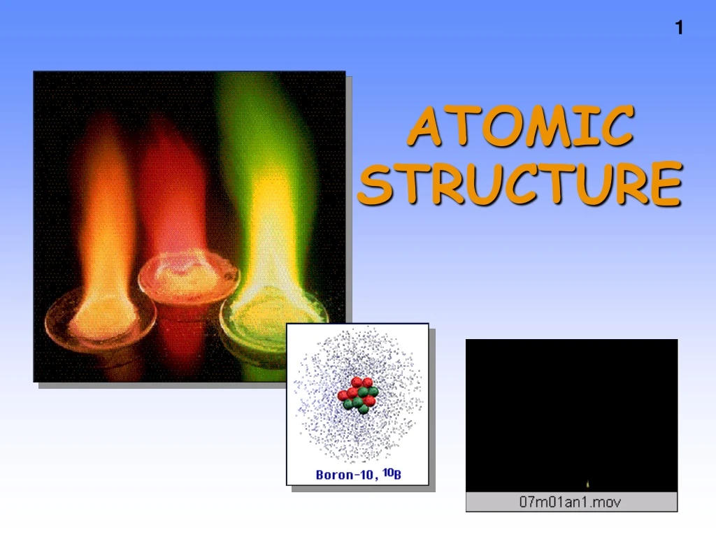
The Electric Pickle • Excited atoms can emit light. • Here the solution in a pickle is excited electrically. The Na+ ions in the pickle juice give off light characteristic of that element.
Atomic Spectra and Bohr The classical view of atomic structure in early 20th century was that an electron (e-) traveled about the nucleus in an orbit. Paradox due to the classical view: 1. Any orbit should be possible and so is any energy. 2. A charged particle moving in an electric field should emit energy. Should end up falling into the nucleus !
Atomic Spectra and Bohr Bohr said classical view was wrong. Needed a new theory — nowadays called OLD QUANTUM THEORY or OLD QUANTUM MECHANICS. e- can exist only in certain discrete orbits — called stationary states. e- is restricted to QUANTIZED energy states. Energy of state = - C/n2 where n = quantum no. = 1, 2, 3, 4, ....
Atomic Spectra and Bohr Energy of quantized state = - C/n2 • Only orbits where n = integral no. are permitted. • Radius of allowed orbitals = n2 • (0.0529 nm) • But note —same eqns. come from a modern quantum mechanics approach. • Results can be used to explain atomic spectra.
Atomic Spectra and Bohr If e-’s are in quantized energy states, then ∆E of states can have only certain values. This explain sharp line spectra.
. n = 2 2 E = - C ( 1 / 2 ) G N R n = 1 E E Y 2 E = - C ( 1 / 1 ) Atomic Spectra and Bohr Calculate ∆E for e- “falling” from a high energy level (n = 2) to a low energy level (n = 1). ∆E = Efinal - Einitial = -C[(1/nf2) - (1/ni)2], when nf=1 and ni=2: ∆E = -(3/4)C Note that the process isEXOTHERMIC ENERGY IS EMITTED AS LIGHT !
wavelength Visible light Amplitude wavelength Node Ultaviolet radiation Electromagnetic Radiation
Electromagnetic Radiation Figure 7.1
Electromagnetic Radiation • Waves have a frequency • Use the Greek letter “nu”, , for frequency, and units are “cycles per sec” • All radiation: • = c • where c = velocity of light = 3.00 x 10⁸ m/sec • Long wavelength --> small frequency • Short wavelength --> high frequency
increasing frequency increasing wavelength Electromagnetic Spectrum Long wavelength --> small frequency Short wavelength --> high frequency
Electromagnetic Radiation Red light has = 700 nm. Calculate the frequency.
. n = 2 2 E = - C ( 1 / 2 ) N R E G E n = 1 Y 2 E = - C ( 1 / 1 ) Atomic Spectra and Bohr ∆E = -(3/4)C C has been found from experiments (and is now called R, the Rydberg constant) R (= C) = 1312 kJ/mol or 3.29 x 10¹⁵ cycles/sec so, E of emitted light = (3/4)R = 2.47 x 10¹⁵ sec-1 and since l = c/n = 121.6 nm This is exactly in agreement with experiment!
Origin of Line Spectra Balmer series Figure 7.12
Atomic Line Spectra and Niels Bohr Bohr’s theory was a great accomplishment. Rec’d Nobel Prize, 1922 Problems with theory — • theory only successful for H. • introduced quantum idea artificially. • So, we go on to • MODERN QUANTUM MECHANICS or WAVE MECHANICS Niels Bohr (1885-1962)
Quantization of Energy Max Planck (1858-1947) Solved the “ultraviolet catastrophe” CCR, Figure 7.5
Quantization of Energy Energy of radiation is proportional to the frequency An object can gain or lose energy by absorbing or emitting radiant energy in QUANTA. E = h • h = Planck’s constant = 6.6262 x 10⁻³⁴ J•s
Photoelectric Effect Experiment demonstrates the particle nature of light.
Photoelectric Effect Classical theory said that E of ejected electron should increase with increase in light intensity—not observed! • No e- observed until light of a certain minimum E is used. • Number of e- ejected depends on light intensity. A. Einstein (1879-1955)
Photoelectric Effect Understand experimental observations if light consists of particles called PHOTONSof discrete energy. PROBLEM: Calculate the energy of 1.00 mol of photons of red light. = 700. nm = 4.29 x 10¹⁴ sec-1
Energy of Radiation Energy of 1.00 mol of photons of red light. E = h• = (6.63 x 10⁻³⁴ J•s)(4.29 x 10¹⁴ sec-1) = 2.85 x 10⁻¹⁹ J per photon E per mol = (2.85 x 10⁻¹⁹ J/ph)(6.02 x 1023 ph/mol) = 171.6 kJ/mol This is in the range of energies that can break bonds.
Quantum or Wave Mechanics de Broglie (1924) proposed that all moving objects have wave properties (mass)(velocity) = h / Note that this relation also applies to electromagnetic radiation: mc = h / , or h = mc , and since E = h and = c / , • E = mc2 • which is Einstein’s famous equation for the relation between mass and energy L. de Broglie (1892-1987)
Quantum or Wave Mechanics Baseball (115 g) at 100 mph = 1.3 x 10⁻³² cm e- with velocity = 1.9 x 108 cm/sec = 0.388 nm Experimental proof of wave properties of electrons
Quantum or Wave Mechanics Schrödinger applied the idea of e- behaving as a wave to the problem of electrons in atoms. He developed the WAVE EQUATION: H = E whose solution gives the so-called WAVE FUNCTION, Describing an allowed state of energy state E Quantization introduced naturally. E. Schrodinger 1887-1961
WAVE FUNCTIONS, • (x)is a function of coordinates, x. • Each corresponds to an ORBITAL — the region of space within which an electron is found. • does NOT describe the exact location of the electron. • 2 is proportional to the probability of finding an e- at a given point.
Uncertainty Principle Problem of defining nature of electrons in atoms solved by W. Heisenberg. Cannot simultaneously define the position and momentum (p= m•v) of an electron: x•p h/(2 ) If we determine the e- velocity, precisely we can not determine the position very well and viceversa. W. Heisenberg 1901-1976
Types of Orbitals d orbital p orbital s orbital
Orbitals • No more than 2 e- assigned to an orbital • Orbitals grouped in s, p, d (and f) subshells s orbitals p orbitals d orbitals
s orbitals p orbitals d orbitals s orbitals p orbitals d orbitals No. orbs. 1 3 5 No. e- 2 6 10
Subshells & Shells • Each shell has a number called thePRINCIPAL QUANTUM NUMBER, n • The principal quantum number of the shell is the number of the period or row of the periodic table where that shell begins.
n = 1 n = 2 n = 3 n = 4 Subshells & Shells
QUANTUM NUMBERS The shape, size, and energy of each orbital is a function of 3 quantum numbers: n (major) ---> shell l (angular) ---> subshell ml(magnetic) ---> designates an orbital within a subshell
QUANTUM NUMBERS Symbol Values Description n (major) 1, 2, 3, ... Orbital size, energy, and # of nodes=n-1 l (angular) 0, 1, 2, ... n-1 Orbital shape or type (subshell) ml (magnetic) -l,...0,...+l Orbital orientation # of orbitals in subshell = 2 l + 1
Shells and Subshells When n = 1, then l = 0 and ml = 0 Therefore, in n = 1, there is 1 type of subshell and that subshell has a single orbital (ml=0 has a single value ---> 1 orbital) This subshell is labeled s (“ess”) Each shell has 1 orbital labeled s, and it is SPHERICALin shape.
s Orbitals All s orbitals are spherical in shape. See Figure 7.14 on page 274 and Screen 7.13.
p Orbitals When n = 2, then l = 0 and l = 1 Therefore, when n = 2 there are 2 types of orbitals — 2 subshells For l = 0 ml = 0, s subshell For l = 1 ml = -1, 0, +1 this is a p subshell with 3 orbitals When l = 1, there is a NODAL PLANE See Screen 7.13
p Orbitals • The three p orbitals are oriented 90o apart in space
3px Orbital 2px Orbital