Download
1 / 31
320 likes | 630 Views
Population Regulation For all these questions about population growth and models describing it, the common observation in nature is that most populations of plants and animals seem to remain fairly constant in size from year to year… An important question in ecology is what mechanisms

E N D
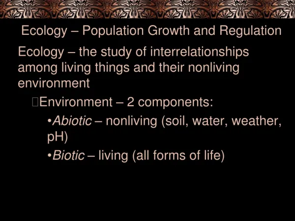
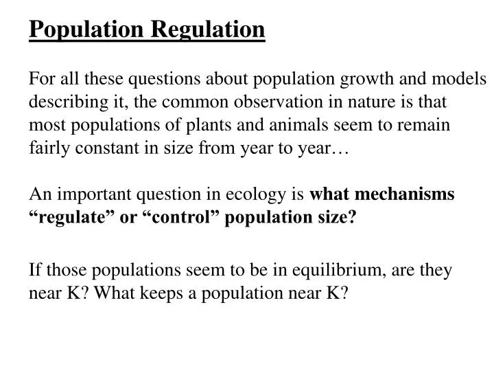
Population Regulation For all these questions about population growth and models describing it, the common observation in nature is that most populations of plants and animals seem to remain fairly constant in size from year to year… An important question in ecology is what mechanisms “regulate” or “control” population size? If those populations seem to be in equilibrium, are they near K? What keeps a population near K?
The most straightforward chain of argument goes… Increased N Resources Become Limiting Competition Among Individuals for Resources Competition has Effects on Birth and Death Rates Does this “regulate” or just limit population size?
What is regulation? The ‘engineering-style’ definition: The amplitude of any perturbation to a variable at its set point will be decreased by regulation to restore the variable to its set point. A practical example: The thermostat in your house is set to a specific temperature (“the set point”). Should temperature in your house increase, the thermostat turns on your central air conditioning to bring the house temperature back down (or vice versa when it becomes to cold and the furnace is turned on).
The idea that populations are “regulated” was highly controversial… There were two opposed schools… David Lack (e.g.1954) argued that population size was regulated by food, predators, and disease, i.e. by biotic factors. Andrewartha & Birch, at around the same time, claimed that numbers were determined by factors extrinsic to the population acting on it. For example, r is strongly affected by weather.
The data used by Andrewartha & Birch came from studies of thrips (Thrips imaginis) growing in roses. They were able to predict population size from past size and weather in the previous fall and current spring fairly well. They found little evidence of density-dependence.
Here are observed and predicted numbers at peak for a number of years, using only previous numbers and weather factors...
They also showed that r was strongly affected by temperature and moisture, key variables in climatic pattern. Climater cool & dry 0.01 cool & moist 0.03 warm & dry 0.01 moderate & moist 0.1
Does this mean that thrips are “regulated” entirely in a density-independent way? The possibility caused a long controversy. For this case, it was largely settled in 1961 by F.E. Smith… What would indicate density-dependence? 1) What happens to per capita growth rate as the population approaches K? Per capita growth rate declines. So should the change per unit time in lnN. Here’s what Smith found in Andrewartha & Birch’s data… (Oct. to Nov. is growth to peak)
2) Smith’s 2nd argument came from variance in population size and growth. A basic principle in statistics is that the variance of a sum of two independent variables should be the sum of the variances of the individual variables, i.e. Var (X + Y) = Var (X) + Var (Y) Look at population growth… ln N(t + 1) = ln N(t) + ln N(t) but in the data the variance is much smaller as the mean N(t) (or ln N(t)) approaches its annual peak. Again, here’s the figure showing that...
For the negative relationship between numbers and the change in numbers as the peak density is approached to be as strong as this, there must have been a strongly negative covariance between the variables (ln N(t) and Δln N(t). That is exactly what would be expected in logistic growth. Growth rate (or Δln N(t)) should decrease as population size increases.
The argument developed, in part, because of the kinds of species studied by supporters of the two points of view... Supporters of Andrewartha & Birch studied insects, for which growth and mortality are strongly affected by weather. Supporters of Lack generally were working with vertebrate species, where behaviour (territory defense) and interactions (competition and predation) often apparently limit population size.
Actually, this long lasting argument should never have occurred. Darwin expressed clearly how both abiotic (density-independent) and biotic (density-dependent) factors interact to determine population size and growth… “Climate plays an important part in determining the average number of species, and periodical seasons of extreme cold or drought seem to be the most effective of all checks…The action of climate seems at first to be quite independent of the struggle for existence; but in so far as climate chiefly acts in reducing food, it brings on the most severe struggle between the individuals, whether of the same or distinct species, which subsist on the same kind of food.”
There are many other examples of apparently density-independent dynamics in populations (many are studies of insects!). In a grain weevil, for example, the intrinsic rate of increase (r) varies 10-fold with minor changes in humidity and temperature in environmental chambers. Wouldn’t we expect insect growth, then, to be sensitive to environmental variation (drought, heavy rainfall, extreme cold or heat) in the real world? In the end, what we consider to be the critical factor depends on the organism we are studying.
When density-dependence occurs, and affects r, those effects are manifest through changes in birth rate and death rate. Here is what the separate relationships look like in abstract form... Intense competition Resources limited Plentiful resources for each individual
The result of changes in both birth and death rates is an equilibrium population size, K. At size K, birth and death rates are equal, i.e. b = d Population size K is called a stable point.
Now let’s compare the birth rate that would be observed when population “regulation” is density-independent versus density-dependent... Birth rate is not a function of density when “regulation” is density-independent. In fact, this shouldn’t be called “regulation”.
And the death rate under each situation... Similarly, when “regulation” is density-independent there is no relationship between death rate and population size or density (and no ‘regulation).
Density-independent birth and death rates tell us that crowding is not important in populations “regulated” in that way. Where population growth is density-independent, there is no tendency for the population to return to an equilibrium value, or K. In fact, K is not defined under those conditions. There is no unique density where b = d, and therefore no equilibrium. So, what might a graph of population size over time look like for a density-independent population? ...
Is there an equilibrium evident? No. Is there a pattern evident? Not with respect to population size.
Organisms showing density-dependent “regulation” of • population size… • appear to have a carrying capacity K • are limited by resources • However, even these species may show changes in • population size near K. • What we observe in some species could be described as • “loose” regulation, and the population is not necessarily • kept close to K. One cause may be environmental variation • altering the effective K. We’ll return to this idea at the end.
In many species, under real environmental conditions • there is no clear regulation of population size because at • the densities occurring in nature birth and death rates are • effectively density-independent. • In these species, patterns of population change are • opportunistic. Populations grow rapidly (exponentially) • when conditions are good. • Exponential growth is followed by large crashes in • numbers when conditions worsen. • This is the pattern usually seen in insects and weedy plants • with annual life cycles.
In some species, population regulation is apparent, and population size fluctuates around K because birth and death rates are density-dependent. The logistic model you have seen and used is one (and literally the simplest) model of density-dependence. The growth rate (effective r) decreases as N increases, due to a decrease in the birth rate and/or an increase in the death rate. The effective r decreases to 0 at population size K. remember dN/dt = rN(K – N/K) effective r = r(K – N/K) Although many other species fit this pattern, it was first described and widely fits data for vertebrate species.
Here are a couple of examples to show you that the model does apply to other populations, as well: An experiment where aphids were introduced onto individual pea plants, and population growth on those pea plants was followed. (Interval between ticks on the x-axis is 2 days.)
These are willows in England after myxamatosis essentially wiped out the population of rabbits that had eaten most seedlings. Thus, here it is not a new population, but one that is starting from small numbers due to removal of predation.
Finally, logistic growth in an ant colony in Brazil. The ants weren’t counted directly, but the size of the colony is directly proportional to the number of craters that surround nest entrances.
In plants, population regulation incorporates a “second level”. In a densely planted population, there is mortality, but the surviving individuals grow. Individual plant weight increases as density decreases. The process is called self-thinning. This figure demonstrates it for horseweed (Erigeron canadensis)
The “trajectory” of plant self-thinning is well established. The slope of a plot of log individual plant weight against log plant density is -3/2. Therefore, self-thinning is called the -3/2 power law. Since plants all follow the same law, plots for much different species follow parallel lines...
Finally,… In still other species, regulation by density-dependent birth and death rates is present, but the regulation is “loose”. When this occurs, population size may depart substantially from K (or K may vary substantially). Such loose regulation occurs when birth and death rates have a range of possible values at any population size. Here we cannot establish a single-valued function relating either/ or birth and death rate to density. This is called “density-vague” regulation.
Here is what you might see as a population trajectory. With density-vague regulation, it may reflect continuous variation in K… or it may reflect density-vague responses in birth and death rates.
How can such variation occur in a regulated population? Here is an abstract view of the ranges of birth and death rates possible plotted over a range of population sizes… K might be any value in the indicated range, i.e. anywhere within the ~diamond shaped box, depending on population size.
References: Andrewartha, H.G. and L.C. Birch (1954) The Distribution and Abundance of Animals. Univ. Chicago Press, Chicago Davidson, J. and H.G. Andrewartha (1948) The influence of rainfall, evaporation and atmospheric temperature on fluctuations in the size of a natural population of Thrips imaginis (Thysanoptera). J. Anim. Ecol. 17:200-222. Lack, D. (1954) The Natural Regulation of Animal Numbers. Oxford Univ. Press, New York, N.Y. Smith, F.E. (1961) Ecology, 42:403-7.