Download
1 / 16
160 likes | 268 Views
Pre-Flare Changes in Current Helicity and Turbulent Regime of the Photospheric Magnetic Field. V.I. Abramenko Big Bear Solar Observatory,NJIT Crimean Astrophysical Observatory, Ukraine Email: avi@bbso.njit.edu. INTRODUCTION. Current helicity

E N D
Pre-Flare Changes in Current Helicity and Turbulent Regime of the Photospheric Magnetic Field V.I. Abramenko Big Bear Solar Observatory,NJIT Crimean Astrophysical Observatory, Ukraine Email: avi@bbso.njit.edu
INTRODUCTION Current helicity Hc=B • ( B) is of particular importance for the problem of DC magnetic energy build-up in the solar atmosphere (Seehafer, 1994): in order to generate a non-zero electromotive force, caused by magnetic field fluctuations (alpha-effect), current helicities of the meanand the fluctuating magnetic field should have opposite signs and the absolute value of current helicity of fluctuations should exceed that of the mean field. Therefore, the necessary condition for alpha-effect to operate is a non-zero imbalance of current helicity. Having vector magnetic field measurements one can estimate a z-related part of the current helicity (Abramenko et al., 1996): hc=Bz• ( B)z
The goal of the present paper • Are parameters of current helicity different before • and after a solar flare? • What aspects of flaring process are reflected in their • variations? In the current study we compare structures of an active region magnetic field observed 2.5-0.5 hours before and 2 minutes after the maximum of a solar flare. For this purpose, we used routines to analyze current helicity and structure functions described in Abramenko et al., 1996; Yurchyshyn et al., 2000; Abramenko, 2002.
OBSERVATIONAL DATA Our data set consists of four high-quality vector magnetograms of an NOAA active region 6757, which had been obtained on August 2, 1991 with the videomagnetograph at HSOS (China, see Wang et al., 1996) 00:36 UT 1st magnetogram 02:00 UT 2nd magnetogram 02:39 UT 3rd magnetogram 03:07 UT start of a 2B/X1.5 flare 03:15 UT peak of a 2B/X1.5 flare 03:17 UT 4th magnetogram 04:07 UT end of 2B/X1.5 flare
Fig. 1. Bz magnetograms and current helicity maps for NOAA AR 6757 obtained on August 2, 1991.
IMBALANCE OF CURRENT HELICITY We calculated the imbalance, h, of current helicity (Fig.2) as the percentage ratio of the net flux of hc to the net flux of moduli of hc (Abramenko et al., 1996). Before the flare, the imbalance h was negative (of about –5 % ) with slowly decreasing absolute value. Predominance of current helicity of certain sign (negative) exists. After the flare maximum the imbalance became a small positive value (of about +1 % ); total positive (negative) helicity decreased by 20 % (27 %). No predominant helicity after the flare maximum. Thus, before the flare the necessary conditions for the alpha-effect were met, whereas after the flare maximum the generation of electromotive force due to fluctuations (alpha-effect) is exhausted.
Fig. 2. Helicity imbalance (blue line ), the cancellation exponent (red line) and GOES X-ray flux (in arbitrary units, green line). The X-ray flux peaks at X1.5.
CANCELLATION EXPONENT To analyze scaling behavior of current helicity we calculated a signed measure: i (r ) = L (r) hc / L(R) hc , where Li (r ) L(R) is a hierarchy of disjoint squares of size r, covering the whole square L(R) , which enclose the active region. Then, we investigated behavior of the alternate in sign, scale by scale, of the measure by defining a cancellation exponent k(Ott et al., 1992): (r ) = L (r) i (r ) r –k
Parameter kis an indication of how rapidly cancellations between negative and positive contributions happen as the spatial scale becomes smaller. The stronger the oscillations of the helicity sing (and, therefore, the strength of tangential discontinuities in the magnetic field), the higher the value of k. Fig.3. Partition functions log(r ) versus log (r/R). The slope of partition function is the cancellation exponent , k, of current helicity
After the flare maximum, at 03:17 UT, the slope of the partition function became smaller than it was before the flare. So, the cancellation exponent ,k, had decreased from 0.75 to 0.66. The decrease of k occurred during a 40 minute time interval during which the flare started and reached its maximum. This means that the strength of tangential discontinuities of the magnetic field was significantly reduced by a flare, which supports Parker’s idea about the principal cause of a solar flare as an avalanche of many small reconnection events (Parker, 1987).
STRUCTURE FUNCTIONS OF Bz Signature of an avalanche can also be recognized in other way, by analyzing the turbulent state of the magnetic field. For turbulence within the inertial range at large magnetic Reynolds numbers, the Bz component of the magnetic field diffuses in exactly the same way as a scalar field (Parker, 1979). Therefore, certain elements of the analysis of turbulent systems can be applied for Bz. In particular, according to a routine proposed recently by Abramenko (2002), we calculated structure functions: S(q) = Bz (x + r ) - Bz( x) q r(q). The scaling exponents (q) are shown in Figure 4.
Fig. 4. Scaling exponents, (q), of structure functions of the order of q versus q, calculated for four magnetograms.
Figure 4 shows that (q) is a concave outward function, whose curvature gradually increases as the active region evolves toward the flare. Such behavior of (q) implies that the multifractality (intermittency) of the Bz component of the magnetic field becomes more complicated. Immediately after the flare maximum the function (q) nearly coincides with the classical Kolmogorov’s straight line, which indicates a monofractal (non-intermittent) structure of the Bz component in the active region. The transition from multifractality to monofractality is a manifestation of an avalanche accompanied by the reduction of small scale tangential discontinuities in the magnetic field (Parker, 2002).
CONCLUSIONS Comparison of current helicity and turbulent state of the magnetic field in an AR before (2.5-0.5 hours) the flare and 2 minutes after the flare maximum allowed us to conclude the following. • Negative imbalance of current helicity of about -5% observed before the • flare became low positive imbalance of about 1 % immediately after • the flare maximum. In the meantime, total positive (negative) helicity • decreased by 20 % (27 %). • The value of the cancellation exponent , k, of current helicity decreased from • 0.75 to 0.66 within a 38 minute time interval during which a flare started • and reached its maximum. • Structure functions of the Bz component of the magnetic field indicated • the transition from intermittent turbulence (multifractality) before the flare • to non-intermittent turbulence (monofractality) after the flare maximum.
Observed changes in current helicity are a manifestation of intrinsic processes in the magnetic field, which drive an active region to a flare. The character of changes supports the following ideas. First, flares are a result of an avalanche of small-scale magnetic reconnection events cascading in a highly stressed magnetic configuration, driven to a critical state by random photospheric motions (Parker, 1987, Charbonneau et al., 2002). Second, the build up of DC magnetic energy in the solar atmosphere due to small scale fluctuations of the magnetic field (alpha-effect, Seehafer, 1994) can take place at least for several hours before a flare.
REFERENCES Abramenko , V.I., Astron. Reports, 46(2), 161-171, 2002. Abramenko, V.I., T.J. Wang, and V.B. Yurchyshyn, Solar Phys., 168, 75-89, 1996. Abramenko, V.I., V.B. Yurchyshyn, and V. Carbone, Solar Phys., 178, 473-476, 1998. Charbonneau, P., S.W. McIntosh, H.L. Liu, and T.J. Bogdan, Solar Phys., 203, 321-353, 2001. Ott, E., Y. Du, K.R. Sreenivasan, A. Juneja, and A.K. Suri, Phys. Rev. Lett., 69, 2654-2657, 1992. Parker, E.N., Cosmical Magnetic Fields, Clarendon Press., Oxford, 1979. Parker, E.N., Solar Phys., 111, 297-308, 1987. Parker, E.N., private communication, 2002. Seehafer, N., Astron. And Astrophys., 284, 593-598, 1994. Wang, J., Z. Shi, H. Wang, and Y. Lu, Astrophys. J., 456, 861-878, 1996. Yurchyshyn, V.B., V.I. Abramenko, and V. Carbone, Astrophys. J., 538, 968-979, 2000.