Download
1 / 45
450 likes | 565 Views
Parameterized Environment Maps. Ziyad Hakura, Stanford University John Snyder, Microsoft Research Jed Lengyel, Microsoft Research. Static Environment Maps (EMs). Generated using standard techniques: Photograph a physical sphere in an environment Render six faces of a cube from object center.

E N D
Parameterized Environment Maps Ziyad Hakura, Stanford University John Snyder, Microsoft Research Jed Lengyel, Microsoft Research
Static Environment Maps (EMs) • Generated using standard techniques: • Photograph a physical sphere in an environment • Render six faces of a cube from object center
Ray-Traced vs. Static EM Self-reflections are missing
3-Step Process • 1) Preprocess:Ray-trace images at each viewpoint • 2) Preprocess:Infer environment maps (EMs) • 3) Run-time:Blend between 2 nearest EMs
Why Parameterized Environment Maps? • Captures view-dependent shading in environment • Accounts for geometric error due to approximation • of environment with simple geometry
How to Parameterize the Space? • Experimental setup • 1D view space • 1˚ separation between views • 100 sampled viewpoints • In general, author specifies parameters • Space can be 1D, 2D or more • Viewpoint, light changes, object motions
Ray-Traced vs. PEM Closely match local reflections like self-reflections
Movement Away from Viewpoint Samples Ray-Traced PEM
Previous Work • Reflections on Planar Surfaces [Diefenbach96] • Reflections on Curved Surfaces [Ofek98] • Image-Based Rendering Methods • Light Field, Lumigraph, Surface Light Field, LDIs • Decoupling of Geometry and Illumination • Cabral99, Heidrich99 • Parameterized Texture Maps [Hakura00]
Surface Light Fields [Miller98,Wood00] Surface Light Field PEM • Dense sampling over • surface points of • low-resolution lumispheres • Sparse sampling over • viewpoints of • high-resolution EMs
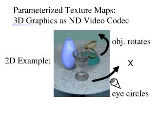
Light View Parameterized Texture Maps [Hakura00] Captures realistic pre-rendered shading effects
Comparison withParameterized Texture Maps • Parameterized Texture Maps [Hakura00] • Static texture coordinates • Pasted-on look away from sampled views • Parameterized Environment Maps • Bounce rays off, intersect simple geometry • Layered maps for local and distant environment • Better quality away from sampled views
EM Representations • EM Geometry • How reflected environment is approximated • Examples: • Sphere at infinity • Finite cubes, spheres, and ellipsoids • EM Mapping • How geometry is represented in a 2D map • Examples: • Gazing ball (OpenGL) mapping • Cubic mapping
Layered EMs • Segment environment into local and distant maps • Allows different EM geometries in each layer • Supports parallax between layers
Distant Local Color Local Alpha Segmented, Ray-Traced Images Fresnel EMs are inferred for each layer separately
Distant Layer Ray directly reaches distant environment
Distant Layer Ray bounces more times off reflector
Distant Layer Ray propagated through reflector
Local Color Local Alpha Local Layer
Fresnel Layer Fresnel modulation is generated at run-time
A x = b HW Filter Coefficients UnknownEM Texels Ray-Traced Image EM Texture Screen Hardware Render EM Inference
Local Alpha Local Color Distant Inferred EMs per Viewpoint
Run-Time • “Over” blending mode to composite local/distant layers • Fresnel modulation, F, generated on-the-fly per vertex • Blend between neighboring viewpoint EMs • Teapot object requires 5 texture map accesses: • 2 EMs (local/distant layers) at each of • 2 viewpoints (for smooth interpolation) and • 1 1D Fresnel map (for better polynomial interpolation)
Video Results • Experimental setup • 1D view space • 1˚ separation between views • 100 sampled viewpoints
Summary • Parameterized Environment Maps • Layered • Parameterized by viewpoint • Inferred to match ray-traced imagery • Accounts for environment’s • Geometry • View-dependent shading • Mirror-like, localreflections • Hardware-accelerated display
Future Work • Placement/partitioning of multiple environment shells • Automatic selection of EM geometry • Incomplete imaging of environment “off the manifold” • Refractive objects • Glossy surfaces
On the Manifold Off the Manifold 2 3 texgen time 35ms 35ms frame time 45ms 57ms FPS 22 17.5 Timing Results #geometry passes
Texture Screen Hardware Render Texel Impulse Response • To measure the hardware impulse response, render with a single texel set to 1.
one column per texel Model for Single Texel one row per screen pixel
Conclusion • PEMs provide: • faithful approximation to ray-traced • images at pre-rendered viewpoint samples • plausible movement away from those samples • using real-time graphics hardware