Download
1 / 46
490 likes | 715 Views
Computer Networks Spring 20 13. Physical Layer (Part 2) Data Encoding Techniques. Interpreting Signals. DCC 9 th Ed. Stallings. Data Encoding Techniques. Digital Data, Analog Signals [ modem ] Digital Data, Digital Signals [ wired LAN ] Analog Data, Digital Signals [ codec ]

E N D
Computer Networks Spring 2013 Physical Layer(Part 2)Data Encoding Techniques
Interpreting Signals DCC 9th Ed. Stallings Computer Networks Data Encoding
Data Encoding Techniques • Digital Data, Analog Signals [modem] • Digital Data, Digital Signals [wired LAN] • Analog Data, Digital Signals [codec] • Frequency Division Multiplexing (FDM) • Wave Division Multiplexing (WDM) [fiber] • Time Division Multiplexing (TDM) • Pulse Code Modulation (PCM) [T1] • Delta Modulation Computer Networks Data Encoding
Analog and Digital Transmissions Figure 2-23.The use of both analog and digital transmissions for a computer-to-computer call. Conversion is done by the modems and codecs. Tanenbaum Computer Networks Data Encoding
Digital Data, Analog Signals [Example – modem] Basis for analog signaling: constant-frequency is a continuous, signal known as thecarrier frequency. Digital data is encoded by modulating one of the three characteristics of the carrier: amplitude, frequency, or phase or some combination of these. Computer Networks Data Encoding
Modulation Techniques DCC 9th Ed. Stallings Computer Networks Data Encoding
Modulation to Keying • Amplitude modulation:: Amplitude Shift Keying (ASK) • Frequency modulation:: • Binary Frequency Shift Keying (BFSK) • Multiple FSK (MFSK) • More than two frequencies used signaling element represents more than one bit. • Phase modulation:: • Binary Phase Shift Keying (BPSK) • Differential* PSK (DPSK) • Quadrature PSK (QPSK) * Explained later Computer Networks Data Encoding
Example 5.4 MFSK DCC 9th Ed. Stallings fc = 250 kHz, fd= 25 kHz M= 8 Frequency assignments: f1= 75 kHz 000 f2= 125 kHz 001 f3 = 175 kHz 010f4= 225 kHz 011 f5= 275 kHz 100f6= 325 kHz 101 f7= 375 kHz 110f8= 425 kHz 111 B = 2Mfd = 400 kHz R = 1/T = 2Lfd = 150 kbps Computer Networks Data Encoding
Modems All advanced modems use a combination of modulation techniquesto transmit multiple bits per baud. Multiple amplitude and multiple phase shifts are combined to transmit several bits per symbol. QPSK (Quadrature Phase Shift Keying) uses four phase shifts per symbol. Modems actually use Quadrature Amplitude Modulation (QAM). These concepts are depicted using constellation points where a point determines a specific amplitude and phase. Computer Networks Data Encoding
Constellation Diagrams (a) QPSK. (b) QAM-16. (c) QAM-64. Figure 2-25. V = 64 v = log2 V = 6 Tanenbaum Computer Networks Data Encoding
Quadrature Amplitude Modulation (QAM) QAM (a combination of ASK and PSK) is used in ADSL and cable modems. Example: QAM-16 = QPSK and QASK Idea - Increase the number of bits transmitted by increasing the number of levels used per symbol. Example: RQAM-64 = 6 RASK Computer Networks Data Encoding
Telephone Modems • Voice grade line ~ 3100 Hz • Nyquist no faster than 6000 baud. • Most modems send at 2400 baud. • To increase data rates, use constellations and error correction-TCM (Trellis Coded Modulation) • Namely, an error correction bit at the physical layer!! Computer Networks Data Encoding
Telephone Modems Tanenbaum V.32 (32 constellation {4 bits} + 1 check bit) 9600 bps V.32bis (6 bits/symbol + 1 check bit) 14,400 bps V.34 (12 bits/symbol) 28,800 bps V.34bis (14 bits/symbol) 33,600 bps thousands of constellation points!! Now we run into Shannon limit based on local loop length and quality of phone lines. Since Shannon limit applies to local loop at both ends, eliminate ISP end local loop. Can now go up to 70 kbps, but now run into Nyquist theorem sampling limits. 4000 Hz (voice grade with guard bands) 8000 samples/sec. with 8 bits per sample (7 useful in US). V.90 and V.92 provide 56-kbps downstream and 33.6-kbps and 48-kbps upstream, respectively. Computer Networks Data Encoding
Digital Data, Digital Signals[the technique used in wired LANs] • Digital signal:: is a sequence of discrete, discontinuous voltage pulses. • Bit duration:: the time it takes for the transmitter to emit the bit. • Issues • Bit timing (sender/receiver clock drift) • Recovery from signal inference • Noise immunity • Error detection {later} • Complexity (cost) Computer Networks Data Encoding
Signal Spectrum Issues • Lack of high frequency components less bandwidth needed for transmission. • DC component direct physical attachment of transmission components {bad}. • Without dc, ac coupling via transformer provides excellent electrical isolation {reduces interference}. • Concentrate transmission power in the middle of the transmission band because channel characteristics worse near band edges. Computer Networks Data Encoding
NRZ ( Non-Return-to-Zero) Codes 1 negative voltage 0 positive voltage Uses two different voltage levels (one positive and one negative) as the signal elements for the two binary digits. NRZ-L ( Non-Return-to-Zero-Level) The voltage is constant during the bit interval. NRZ-Lis used for short distances between a terminal and modem or terminal and computer. Computer Networks Data Encoding
NRZ ( Non-Return-to-Zero) Codes NRZ-I ( Non-Return-to-Zero-Invert on ones) The voltage is constant during the bit interval. NRZI is a differential encodingscheme (i.e., the information transmitted is terms ofcomparing adjacent signal elements.) 1 existence of a signal transitionat the beginning of the bit time (either a low-to-high or a high-to-low transition) 0 no signal transition at the beginning of the bit time Computer Networks Data Encoding
Bi–Phase Codes Bi-phase codes– require at least one transition per bit time and may have as many as two transitions. • the maximum modulation rate is twice that of NRZ greater transmission bandwidth is required. Advantages: Synchronization – with a predictable transition per bit time the receiver can “synch” on the transition [self-clocking]. No d.c. component. Error detection – the absence of an expected transition can be used to detect errors. Computer Networks Data Encoding
Manchester Encoding • There is always a mid-bit transition {which is used as a clocking mechanism}. • The direction of the mid-bit transition represents the digital data. Consequently, there may be a second transition at the beginning of the bit interval. Used in 802.3 baseband coaxial cable and CSMA/CD twisted pair. Some textbooks disagree on this definition!! 1 low-to-high transition 0 high-to-low transition Computer Networks Data Encoding
Differential Manchester Encoding • mid-bit transition is ONLY for clocking. Differential Manchester is both differential and bi-phase. Note – the coding convention for DifferentialManchester is the opposite convention from NRZI. Used in 802.5 (token ring) with shielded twisted pair. * Modulation rate for Manchester and Differential Manchester is twicethe data rate inefficient encoding for long-distance applications. 1 absence of transition at the beginning of the bit interval 0 presence of transitionat the beginning of the bit interval Computer Networks Data Encoding
Bi-Polar Encoding 1 alternating +1/2 , -1/2 voltage 0 0 voltage • Has the same issues as NRZI for a long string of 0’s. • A systemic problem with polar is the polarity can be backwards. Computer Networks Data Encoding
Digital Encoding Techniques 1 0 1 1 1 1 0 0 0 Unipolar NRZ Polar NRZ NRZ-Inverted (Differential Encoding) Leon-Garcia & Widjaja: Communication Networks Bipolar Encoding Manchester Encoding Differential Manchester Encoding Computer Networks Data Encoding
Analog Data, Digital Signals[Example – PCM (Pulse Code Modulation)] The most common technique for using digital signals to encode analog data is PCM. Example: To transfer analog voice signals off a local loop to digital end office within the phone system, one uses a codec. Because voice data limited to frequencies below 4000 HZ, a codec makes 8000 samples/sec. (i.e., 125 microsec/sample). Computer Networks Data Encoding
Multiplexing Multiplexing {general definition} :: Sharing a resource over time. (a) (b) A A A A Trunk group B B B B MUX MUX C C C C Leon-Garcia & Widjaja: Communication Networks Computer Networks Data Encoding
Example: 4 users FDM frequency time TDM frequency time Frequency Division Multiplexing (FDM) vs Time Division Multiplexing (TDM) K & R Computer Networks Data Encoding
A f H 0 B f 0 H C B A f C f 0 H Frequency Division Multiplexing (a) Individual signals occupy H Hz (b) Combined signal fits into channel bandwidth Leon-Garcia & Widjaja: Communication Networks Computer Networks Data Encoding
Frequency Division Multiplexing Figure 2-31.(a) The original bandwidths. (b) The bandwidths raised in frequency. (c) The multiplexed channel. Tanenbaum Computer Networks Data Encoding
Wavelength Division Multiplexing Wavelength division multiplexing. Figure 2-32. Tanenbaum Computer Networks Data Encoding
Time Division Multiplexing Computer Networks Data Encoding
Concentrator [Statistical Multiplexing] Computer Networks Data Encoding
Statistical Multiplexing DCC 9th Ed. Stallings Computer Networks Data Encoding
T1 System A A B MUX MUX B 22 23 24 1 b 24 2 b . . . C C frame Leon-Garcia & Widjaja: Communication Networks Computer Networks Data Encoding
T1 - TDM Link The T1 carrier (1.544 Mbps). Figure2-33.T1 Carrier (1.544Mbps) Tanenbaum Computer Networks Data Encoding
Pulse Code Modulation (PCM) T1 example for voice-grade input lines: implies both codex conversion of analog to digital signals (PCM) and TDM. Computer Networks Data Encoding
Analog Data, Digital Signals • digitization is conversion of analog data into digital data which can then: • be transmitted using NRZ-L. • be transmitted using code other than NRZ-L (e.g., Manchester encoding). • be converted to analog signal. • analog to digital conversion done using a codec: • pulse code modulation • delta modulation DCC 9th Ed. Stallings Computer Networks Data Encoding
Digitizing Analog Data DCC 9th Ed. Stallings Computer Networks Data Encoding
Pulse Code Modulation Stages DCC 9thEd. Stallings Computer Networks Data Encoding
Pulse Code Modulation (PCM) • Analog signal is sampled. • Converted to discrete-time continuous-amplitude signal (Pulse Amplitude Modulation). • Pulses are quantized and assigned a digital value. • A 7-bit sample allows 128 quantizing levels. Computer Networks Data Encoding
Pulse Code Modulation (PCM) • PCM uses non-linear encoding, i.e., amplitude spacing of levels is non-linear. • There is a greater number of quantizing steps for low amplitude. • This reduces overall signal distortion. • This introduces quantizing error (or noise). • PCM pulses are then encoded into a digital bit stream. • 8000 samples/sec x 7 bits/sample = 56 Kbps for a single voice channel. • 7-bit codes 128 quantization levels Computer Networks Data Encoding
PCM Stages DCC 9thEd. Stallings Computer Networks Data Encoding
PCM Nonlinear Quantization DCC 9thEd. Stallings Computer Networks Data Encoding
Delta Modulation (DM) • The basic idea in delta modulation is to approximate the derivative of analog signal rather than its amplitude. • The analog data is approximated by a staircase function that moves up or down by one quantization level at each sampling time. output of DM is a single bit. • PCM preferred because of better SNR characteristics. Computer Networks Data Encoding
Delta Modulation DCC 9thEd. Stallings Computer Networks Data Encoding
Digital Techniques for Analog Data • Continue to grow in popularity because: • Repeaters used instead of amplifiers. • TDM used for digital signals (e.g. SONET). • Digital signaling allows more efficient digital switching techniques. • More efficient codes developed (e.g. interframe coding techniques for video). Example color TV – uses 10-bit codes 4.6 MHZ bandwidth signal yields 92Mbps. Computer Networks Data Encoding
Data Encoding Summary • Digital Data, Analog Signals [modem] • Three forms of modulation (amplitude, frequency and phase) used in combination to increase the data rate. • Constellation diagrams (QPSK and QAM) • Digital Data, Digital Signals [wired LANs] • Tradeoffs between self clocking and required frequency. • Biphase, differential, NRZL, NRZI, Manchester, differential Manchester, bipolar. Computer Networks Data Encoding
Data Encoding Summary • Analog Data, Digital Signals [codec] • Multiplexing Detour: • Frequency Division Multiplexing (FDM) • Wave Division Multiplexing (WDM) [fiber] • Time Division Multiplexing (TDM) • Statistical TDM (Concentrator) • Codex functionality: • Pulse Code Modulation (PCM) • T1 line {classic voice-grade TDM} • PCM Stages (PAM, quantizer, encoder) • Delta Modulation Computer Networks Data Encoding