Download
1 / 39
410 likes | 1.3k Views
OPS 301 Module B and Additional Topics in Linear Programming. Dr. Steven Harrod. Topics. Definition of Linear Programming Applications Mathematical Requirements Linear functions Convex, non-negative feasible region Single objective Steps to Formulate a Problem Solution Techniques

E N D
OPS 301Module B andAdditional Topics inLinear Programming Dr. Steven Harrod
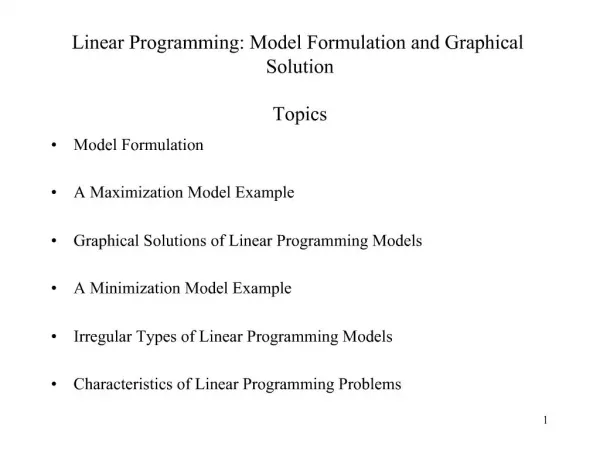
Topics • Definition of Linear Programming • Applications • Mathematical Requirements • Linear functions • Convex, non-negative feasible region • Single objective • Steps to Formulate a Problem • Solution Techniques • Graphical • Simplex
Linear Programming • A mathematical tool to make multiple decisions affecting a single outcome or objective • Guaranteed to find the optimal solution (best possible set of decisions) relative to the stated objective and linear assumptions
LP Applications • Selecting the product mix in a factory to make best use of machine- and labor-hours available while maximizing the firm’s profit • Determining the best diet for persons or animals based on any combination of nutrition, cost, taste, etc. • Determining production, routes, and storage locations that will minimize total shipping cost
Requirements of an LP Problem • Linear • Acceptable: X1, 2X2, 9 • Not acceptable: X2, X3, |X|, √X • Convex A line drawn between any two points on the region will not travel outside the region • Single Objective
Convex and Linear X2 – – 80 – – 60 – – 40 – – 20 – – – Feasible region | | | | | | | | | | | 0 20 40 60 80 100 X1
Linear, But Not Convex X2 – – 80 – – 60 – – 40 – – 20 – – – Feasible region | | | | | | | | | | | 0 20 40 60 80 100 X1
Convex, But Not Linear X2 – – 80 – – 60 – – 40 – – 20 – – – Feasible region | | | | | | | | | | | 0 20 40 60 80 100 X1
Formulating an LP • What is the goal? • “Objective Function” • Maximize – make as large as possible • Minimize – make as small as possible • What do you control? • Called “Decision Variables” • Must be non-negative • What are the limits? • Resources not to exceed (<=) • Minimum requirements to meet (>=) • Items that must be used/served exactly (=) • Constraints are labeled “s.t.” for “subject to”
Example Young MBA Erica Cudahy may invest up to $1,000. She can invest her money in stocks and loans. Each dollar invested in stocks yields 10¢ profit, and each dollar invested in a loan yields 15¢ profit. At least 30% of all money invested must be in stocks, and at least $400 must be in loans. source: Winston, Operations Research, 2004
Example • What is the goal? Maximize profit. • What do we control? Dollar amount invested each in stocks and loans. • What are the limits? • At least $400 invested in loans • 30% invested in stocks • $1000 maximum available to invest
Mathematical Formulation • Label our decision variables • X1 dollar amount invested in stocks • X2 dollar amount invested in loans • Write objective function • the value resulting from our decisions • 0.10 X1 + 0.15 X2
Mathematical Formulation • Write Limits • $1000 available to invest X1 + X2 <= 1000 • at least 30% of all money in stocks 0.3 (X1 + X2) <= X1 • Arrange all variables on left side • – 0.7 X1 + 0.3 X2 <=0 • at least $400 in loans X2 >=400
Complete Formulation max 0.10 X1 + 0.15 X2 s.t. X1 + X2 <= 1000 – 0.7 X1 + 0.3 X2 <=0 X2 >=400 X1, X2 >=0
Graphical Solution • Can be used when there are two decision variables • Plot the constraint equations at their limits by converting each equation to an equality • Identify the feasible solution space • Create an iso-profit line based on the objective function • Move this line outwards until the optimal point is identified
Graphical Example max 7 X1 + 5 X2 s.t. 4X1 + 3X2 ≤ 240 2X1 + 1X2 ≤ 100 X1, X2 >=0
2X1 + 1X2 ≤ 100 4X1 + 3X2 ≤ 240 Graphical Solution X2 – – 80 – – 60 – – 40 – – 20 – – – Feasible region | | | | | | | | | | | 0 20 40 60 80 100 X1 Figure B.3
X2 – – 80 – – 60 – – 40 – – 20 – – – Choose a possible value for the objective function Assembly (constraint B) $210 = 7X1 + 5X2 Solve for the axis intercepts of the function and plot the line Number of Watch TVs Electronics (constraint A) X2 = 42 X1 = 30 Feasible region | | | | | | | | | | | 0 20 40 60 80 100 X1 Figure B.3 Number of Walkmans Graphical Solution Iso-Profit Line Solution Method
$210 = $7X1 + $5X2 (30, 0) Graphical Solution X2 – – 80 – – 60 – – 40 – – 20 – – – (0, 42) | | | | | | | | | | | 0 20 40 60 80 100 X1 Figure B.4
$210 = $7X1 + $5X2 $350 = $7X1 + $5X2 $280 = $7X1 + $5X2 $420 = $7X1 + $5X2 Graphical Solution X2 – – 80 – – 60 – – 40 – – 20 – – – | | | | | | | | | | | 0 20 40 60 80 100 X1 Figure B.5
Maximum profit line Optimal solution point (X1 = 30, X2 = 40) $410 = $7X1 + $5X2 Graphical Solution X2 – – 80 – – 60 – – 40 – – 20 – – – | | | | | | | | | | | 0 20 40 60 80 100 X1 Figure B.6
2 3 1 4 Corner-Point Method X2 – – 80 – – 60 – – 40 – – 20 – – – | | | | | | | | | | | 0 20 40 60 80 100 X1 Figure B.7
Point 1 : (X1 = 0, X2 = 0) Profit $7(0) + $5(0) = $0 Point 2 : (X1 = 0, X2 = 80) Profit $7(0) + $5(80) = $400 Point 4 : (X1 = 50, X2 = 0) Profit $7(50) + $5(0) = $350 Corner-Point Method • The optimal value will always be at a corner point • Find the objective function value at each corner point and choose the one with the highest profit
4X1 + 3X2 ≤ 240 (electronics time) 2X1 + 1X2 ≤ 100 (assembly time) 4X1 + 3X2 = 240 - 4X1 - 2X2 = -200 + 1X2 = 40 Point 1 : (X1 = 0, X2 = 0) Profit $7(0) + $5(0) = $0 Point 2 : (X1 = 0, X2 = 80) Profit $7(0) + $5(80) = $400 Point 4 : (X1 = 50, X2 = 0) Profit $7(50) + $5(0) = $350 Corner-Point Method • The optimal value will always be at a corner point • Find the objective function value at each corner point and choose the one with the highest profit Solve for the intersection of two constraints 4X1 + 3(40) = 240 4X1 + 120 = 240 X1 = 30
Point 1 : (X1 = 0, X2 = 0) Profit $7(0) + $5(0) = $0 Point 2 : (X1 = 0, X2 = 80) Profit $7(0) + $5(80) = $400 Point 4 : (X1 = 50, X2 = 0) Profit $7(50) + $5(0) = $350 Point 3 : (X1 = 30, X2 = 40) Profit $7(30) + $5(40) = $410 Corner-Point Method • The optimal value will always be at a corner point • Find the objective function value at each corner point and choose the one with the highest profit
Beyond 2 Variables,Matrix Algebra • To solve problems of more than two variables with more complex feasible regions (decimal and fractional values) requires computers and matrix algebra • Matrix algebra allows easy calculation of corner points • Simplex method finds optimal corner point
Matrix Algebra max 7 X1 + 5 X2 s.t. 4X1 + 3X2 ≤ 240 2X1 + 1X2 ≤ 100 X1, X2 >=0 Define 4 matrices:
Matrix Formulation max cx s.t. Ax <=b x>=0
Linear System Solution • IF Ax=b, and A is “Square” (number of rows equals number of columns) • DEFINE the inverse of A: A-1 • THEN x=A-1b • Use spreadsheet to calculate inverse • How to convert Ax<=b to Ax=b?
Slack Variables “S” max 7 X1 + 5 X2 + 0 S1 + 0 S2 s.t. 4X1 + 3X2 + S1 = 240 2X1 + 1X2 + S2 = 100 {one of X1, X2, S1, S2} = 0 {one of X1, X2, S1, S2} = 0 X1, X2, S1, S2 >=0
Instructions for Slack • Add one new slack variable to each constraint • Slack variables added to objective with zero coefficient • Square matrix by choosing some variables equal to zero
Slack Variables “S” New matrices:
Solution Method • Type all of these matrices into Excel • In each row of ? • Enter a single 1 • Fill the rest of the row with zeros • Do not put 1 in same column on multiple rows • Do not leave cells blank, zeros are required • Label matrix “x” your corner point
Solution Method • Select the cells of the corner point • Enter formula =mmult(minverse(A matrix cells), b matrix cells) • Keep all cells selected • Hold keys ctrl & shift, then press Enter. • If successful, number values should display in corner point • Pick a new cell • Label “Objective Value” • Enter formula =mmult(c matrix cells, corner point cells) • Again hold keys ctrl & shift, then press enter
Finding Corner Points • Select different combinations of variables to set to zero by moving 1 value within row • Round corner points to 3 decimals (#.###) • Ignore corner points found with negative values • Objective value calculated is value given displayed choices or decisions for variables • Given all combinations, all possible corner points, the optimal solution will be one of these
Simplex Method • Realistic problems quickly grow to have more corner points than humanly possible to examine • Simplex method starts from a simple point and jumps from point to point until reaching optimal, then stops. • Does not usually need to cover a large number of points • Solution can be proven optimal without listing all corner points • Developed by George Dantzig in the late 1940s • Most computer-based LP packages use the simplex method
Simplex Spreadsheet • Simplex spreadsheet provided for you • Follow instructions on spreadsheet • Simplex method uses additional matrix algebra to calculate a directional indicator to next best corner point • Simplex also uses matrix algebra to identify stopping point
Conclusion • Understand • Use of LP • Mathematical Requirements • Steps to Formulate a Problem • Solution Techniques • Graphical • Simplex • Matrix Algebra Foundation ofAdvanced Work