Download
1 / 35
860 likes | 1.73k Views
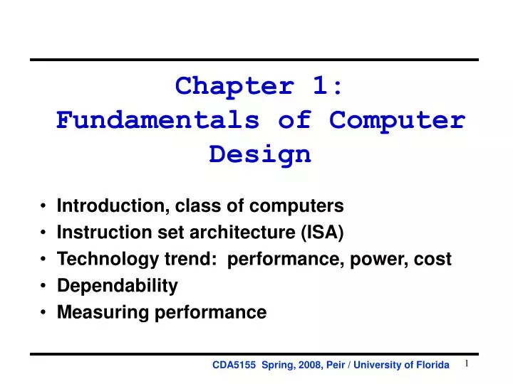
Chapter 1: Fundamentals of Computer Design. Introduction, class of computers Instruction set architecture (ISA) Technology trend: performance, power, cost Dependability Measuring performance. CDA5155 Spring, 2008, Peir / University of Florida. Microprocessor Performance Trends.

E N D
Chapter 1: Fundamentals of Computer Design Introduction, class of computers Instruction set architecture (ISA) Technology trend: performance, power, cost Dependability Measuring performance CDA5155 Spring, 2008, Peir / University of Florida
Conventional Wisdom • Old CW: Uniprocessor performance 2X / 1.5 yrs • New CW: Power Wall + ILP Wall + Memory Wall • = New Brick Wall Uniprocessor performance now 2X / 5(?) yrs • Sea change in chip design: multiple “cores” (2X processors per chip / ~ 2 years) • More simpler processors are more power efficient • Exploit TLP and DLP, not ILP • Programmer / compiler involvement
Classes of Computers • Desk top • Still largest market in dollar amount • Driven by price-performance • Application-driven performance evaluation • Server • High performance, high power • Availability, scalability • Designed for efficient throughput • Embedded system • Largest volume • Real-time performance requirement • Minimize memory and power
Computer Architecture • Old Definition • Old definition of computer architecture = instruction set design • Other aspects of computer design called implementation • Insinuates implementation is uninteresting or less challenging • Right view is computer architecture >> ISA • Architect’s job much more than instruction set design; technical hurdles today more challenging than instruction set design • New Definition • What really matters is the functioning of the complete system • hardware, runtime system, compiler, operating system, application • In networking, called the “End to End argument” • Computer architecture is not just about transistors, individual instructions, or particular implementations • E.g., RISC replaced complex instr. with compiler + simple instr.
ISA • An instruction set architecture is a specification of a standardized programmer-visible interface to hardware, comprised of: • A set of instructions (instruction types and operations) • With associated argument fields, assembly syntax, and machine encoding. • A set of named storage locations and addressing • Registers, memory, … Programmer-accessible caches? • A set of addressing modes (ways to name locations) • Types and sizes of operands • Control flow instructions • Often an I/O interface (usually memory-mapped)
Example: MIPS r0 r1 ° ° ° r31 0 Programmable storage 2^32 x bytes 31 x 32-bit GPRs (R0=0) 32 x 32-bit FP regs (paired DP) HI, LO, PC Data types ? Format ? Addressing Modes? PC lo hi • Arithmetic logical • Add, AddU, Sub, SubU, And, Or, Xor, Nor, SLT, SLTU, • AddI, AddIU, SLTI, SLTIU, AndI, OrI, XorI, LUI • SLL, SRL, SRA, SLLV, SRLV, SRAV • Memory Access • LB, LBU, LH, LHU, LW, LWL,LWR • SB, SH, SW, SWL, SWR • Control • J, JAL, JR, JALR • BEq, BNE, BLEZ,BGTZ,BLTZ,BGEZ,BLTZAL,BGEZAL 32-bit instructions on word boundary
Overview of This Course • Understanding the design techniques, machine structures, technology factors, evaluation methods that determine the form of computers in 21st Century Parallelism Technology Programming Languages Applications Interface Design (ISA) Computer Architecture: • Organization • Hardware/Software Boundary Compilers Operating Measurement & Evaluation History Systems
Technology Trend • Drill down into 4 technologies: • Disks, • Memory, • Network, • Processors • Compare ~1980 vs. ~2000 • Performance Milestones in each technology • Compare for Bandwidth vs. Latency improvements in performance over time • Bandwidth: number of events per unit time • E.g., M bits / second over network, M bytes / second from disk • Latency: elapsed time for a single event • E.g., one-way network delay in microseconds, average disk access time in milliseconds
CDC Wren I, 1983 3600 RPM 0.03 GBytes capacity Tracks/Inch: 800 Bits/Inch: 9550 Three 5.25” platters Bandwidth: 0.6 MBytes/sec Latency: 48.3 ms Cache: none Disk Comparison • Seagate 373453, 2003 • 15000 RPM (4X) • 73.4 GBytes (2500X) • Tracks/Inch: 64000 (80X) • Bits/Inch: 533,000 (60X) • Four 2.5” platters (in 3.5” form factor) • Bandwidth: 86 MBytes/sec (140X) • Latency: 5.7 ms (8X) • Cache: 8 MBytes
1980 DRAM(asynchronous) 0.06 Mbits/chip 64,000 xtors, 35 mm2 16-bit data bus per module, 16 pins/chip 13 Mbytes/sec Latency: 225 ns (no block transfer) Memory Comparison • 2000Double Data Rate Synchr. (clocked) DRAM • 256.00 Mbits/chip (4000X) • 256,000,000 xtors, 204 mm2 • 64-bit data bus per DIMM, 66 pins/chip (4X) • 1600 Mbytes/sec (120X) • Latency: 52 ns (4X) • Block transfers (page mode)
"Cat 5" is 4 twisted pairs in bundle Twisted Pair: Copper, 1mm thick, twisted to avoid antenna effect LAN Comparison • Ethernet 802.3 • Year of Standard: 1978 • 10 Mbits/s link speed • Latency: 3000 msec • Shared media • Coaxial cable • Ethernet 802.3ae • Year of Standard: 2003 • 10,000 Mbits/s (1000X)link speed • Latency: 190 msec (15X) • Switched media • Category 5 copper wire Plastic Covering Braided outer conductor Insulator Copper core
CPU Comparison • 2001 Intel Pentium 4 • 1500MHz (120X) • 4500 MIPS (peak) (2250X) • Latency 15 ns (20X) • 42,000,000 xtors, 217 mm2 • 64-bit data bus, 423 pins • 3-way superscalar,Dynamic translate to RISC, Superpipelined (22 stage),Out-of-Order execution • On-chip 8KB Data caches, 96KB Instr. Trace cache, 256KB L2 cache • 1982 Intel 80286 • 12.5 MHz • 2 MIPS (peak) • Latency 320 ns • 134,000 xtors, 47 mm2 • 16-bit data bus, 68 pins • Microcode interpreter, separate FPU chip • (no caches)
Bandwidth vs. Latency • Performance Milestones: • Processor: ‘286, ‘386, ‘486, Pentium, Pentium Pro, Pentium 4 (21x,2250x) • Ethernet: 10Mb, 100Mb, 1000Mb, 10000 Mb/s (16x,1000x) • Memory Module: 16bit plain DRAM, Page Mode DRAM, 32b, 64b, SDRAM, DDR SDRAM (4x,120x) • Disk : 3600, 5400, 7200, 10000, 15000 RPM (8x, 143x)
Summary on Technology Trend • For disk, LAN, memory, and microprocessor, bandwidth improves by square of latency improvement • In the time that bandwidth doubles, latency improves by no more than 1.2X to 1.4X • Lag probably even larger in real systems, as bandwidth gains multiplied by replicated components • Multiple processors in a cluster or even in a chip • Multiple disks in a disk array • Multiple memory modules in a large memory • Simultaneous communication in switched LAN • HW and SW developers should innovate assuming Latency Lags Bandwidth • If everything improves at the same rate, then nothing really changes • When rates vary, require real innovation
Define and Quantity Power • For CMOS, traditional dominant energy consumption • has been in switching transistors, called dynamic power • For mobile devices, energy better metric • For fixed task, slowing clock rate (frequency switched) • reduces power, but not energy • Capacitive load, a function of number of transistors • connected to output and technology, which determines • capacitance of wires and transistors • Dropping voltage helps both, so went from 5V to 1V • Turn off clock to save energy & dynamic power
Example • Suppose 15% reduction in voltage results in a 15% • reduction in frequency. What is impact on dynamic • power?
Static Power • Because leakage current flows even when a • transistor is off, now static power important too • Leakage current increases in processors with • smaller transistor sizes • Increasing the number of transistors increases • power even if they are turned off • In 2006, goal for leakage is 25% of total power • consumption; high performance designs at 40% • Very low power systems even gate voltage to • inactive modules to control loss due to leakage
Define and Quantity Dependability • How decide when a system is operating properly? • Infrastructure providers now offer Service Level Agreements (SLA) to guarantee that their networking or power service would be dependable • Systems alternate between 2 states of service with respect to an SLA: • Service accomplishment, where the service is delivered as specified in SLA • Service interruption, where the delivered service is different from the SLA • Failure = transition from state 1 to state 2 • Restoration = transition from state 2 to state 1
Dependability (cont.) • Module reliability = measure of continuous service accomplishment (or time to failure).2 metrics: • Mean Time To Failure (MTTF) measures Reliability • Failures In Time (FIT) = 1/MTTF, the rate of failures • Traditionally reported as failures per billion hours of operation • Mean Time To Repair (MTTR) measures Service Interruption • Mean Time Between Failures (MTBF) = MTTF+MTTR • Module availability measures service as alternate between the 2 states of accomplishment and interruption (number between 0 and 1, e.g. 0.9) • Module availability = MTTF / ( MTTF + MTTR)
Example • If modules have exponentially distributed lifetimes (age of module does not affect probability of failure), overall failure rate is the sum of failure rates of the modules • Calculate FIT and MTTF for 10 disks (1M hour MTTF per disk), 1 disk controller (0.5M hour MTTF), and 1 power supply (0.2M hour MTTF): 17,000 failure per billion hours
Performance Measurement • Performance metrics: execution time • Other metrics • Wall-clock time, response time, elapsed time • CPU time: user or system • We will focus on CPU performance, i.e. user CPU time on unloaded system
Benchmark Suites • Desktop • New SPEC CPU2006 (Fig. 1.13) • SPEC CPU2000: 11 integer, 14 floating-point • SPECviewperf, SPECapc: graphics benchmarks • Server • SPEC CPU2000: running multiple copies, SPECrate • SPECSFS: for NFS performance • SPECWeb: Web server benchmark • TPC-x: measure transaction-processing, queries, and decision making database applications • Embedded Processor • New area • EEMBC: EDN Embedded Microprocessor Benchmark Consortium
Comparing Performance • Arithmetic Mean: • Weighted Arithmetic Mean: • Geometric Mean: • Execution time ratio is normalized to a base machine • Is used to figure out SPECrate
SPECRatio • SPECRatio: Normalize execution times to reference computer, yielding a ratio proportional to performance = • time on reference computer • time on computer being rated • If program SPECRatio on Computer A is 1.25 • times bigger than Computer B, then
Summarize Suite Performance • Since ratios, proper mean is geometric mean (SPECRatio unitless, so arithmetic mean meaningless) • Geometric mean of the ratios is the same as the ratio of the geometric means • Ratio of geometric means = Geometric mean of performance ratios choice of reference computer is irrelevant! • These two points make geometric mean of ratios attractive to summarize performance
Amdahl’s Law • Where: • f is a fraction of the execution time that can be enhanced • n is the enhancement factor • Example: f = .9, n = 10 => Speedup = 5.26
CPU Performance Equation • Clock Cycle Time: Hardware technology and organization • CPI: Organization and Inst Set Architecture (ISA) • Instruction Count: ISA and compiler technology • We will focus more on the organization issues
Example • Parameters: • FP operations (including FPSQR) = 25% • CPI for FP operations = 4; CPI for others = 1.33 • Frequency of FPSQR = 2%; CPI of FPSQR = 20 • Compare the following 2 designs: • Decrease CPI of FPSQR to 2; or CPI of all FP to 2.5
Misc. Items • Check SPEC web site for more information, http://www.spec.org • Read Fallacies and Pitfalls • For example, MIPS is an accurate measure for comparing performance among computers is a Fallacy
Example Using MIPS • Instruction distribution: • ALU: 43%, 1 cycle/inst • Load: 21%, 2 cycle/inst • Store: 12%, 2 cycle/inst • Branch: 24%, 2 cycle/inst • Optimization compiler reduces 50% of ALU