Download
1 / 21
210 likes | 354 Views
Comparison between Forecasting and Retrospective Air Quality Simulations of 2006 TexAQS-II. Daewon W. Byun* D.-G. Lee, F. Ngan, H.-C. Kim, B. Czader Arastoo Biazar (UAH) B. Rappenglueck, B. Lefer Postdocs & Students University of Houston Institute for Multidimensional Air Quality Studies

E N D
Comparison between Forecasting and Retrospective Air Quality Simulations of 2006 TexAQS-II Daewon W. Byun* D.-G. Lee, F. Ngan, H.-C. Kim, B. Czader Arastoo Biazar (UAH) B. Rappenglueck, B. Lefer Postdocs & Students University of Houston Institute for Multidimensional Air Quality Studies * Present Affiliation: Air Resources Laboratory, NOAA
Governing Equation and Inputs Affecting AQF Results Quality of forecasting depends on both model formulations and inputs. For AQF, daily meteorology is the main driver but IC, BC, and emissions can affect forecasting quality as well. Demonstrate how AQF can be affected by wind & cloud (photolysis), emissions, and IC
Reduce AQ modeling biases by improving meteorology through data assimilation? Emissions & Flow direction Missing rain, lingering effects (MET?) Missing rain O3 (EI) (IC) (TS) (TS) Rain/cloud not correct Too little cloud Low pm PBL over G-Bay (BC?) High bgrnd O3, southerly flow (PBL/SST?) Bogus LA plume (BC?) O3 averaged over the CAMS sites in the HGB domain for Aug. 16-Sept. 14, 2006 (upper) and Sept. 15 – Oct. 6, 2006 period (lower).
D36 MM5 Configuration for Forecasting Simulation period: August 23 – September 9, 2006 Model was initialized every 2 days and each run was 54 hours long. The first 6 hours was not used for air quality modeling. Thick lines: MM5 domain,Thin lines: CMAQ domain E12 E04
MUltiscale Nest-down Data Assimilation System (MUNDAS) • Utilizes existing objective analysis and nudging tools in the MM5 system. • Incorporate extensive OBS available in the simulated domain for the retrospective simulation of the TexAQS-II period. • Update SFC characteristics inputs in MM5 with satellite observation-based land use/land cover (UT-CSR and TFS) and sea surface temperature (GOES). CAMS: surface met., only in TX, concentrating in big city MADIS: surface – METARS & Buoy etc. upper level – NPN, aircraft sounding & radiosonde Updated LULC for E04 + Difference plot of vegetation fraction Updated - Original
Flow direction Missing rain, lingering effects Missing rain Rain/cloud not correct Too little cloud / wrong place Flow direction/speed Forecast vs. Retrospective Met – impact on AQF U (westerly) component Westerly wind component averaged over the CAMS sites in the HGB domain for Aug. 16-Sept. 14, 2006 (upper) and Sept. 15 – Oct. 6, 2006 period (lower).
Forecasting vs. Retrospective Meteorology Relative Humidity (RH) daytime humidity – very little bias except for the rainy days Nighttime humidity biases – related with thick model layer Relative humidity averaged over the CAMS sites in the HGB domain for Aug. 16-Sept. 14, 2006 (upper) and Sept. 15 – Oct. 6, 2006 period (lower).
Forecasting vs. RetrospectiveMM5 Simulation 1.5 m temperature No improvement improved Still problematic..rain Worse… rain improved improved improved improved improved improved Rain? Cloud problem? 1.5 m temperature averaged over the CAMS sites in the HGB domain for Aug. 16-Sept. 14, 2006 (upper) and Sept. 15 – Oct. 6, 2006 period (lower).
Impact of assimilated wind on CMAQ simulation: Episode August 31, 2006 Time series of wind vector at CAMS sites on 8/31 (black: MM5, red: OBS) AQF assimilated AQF O3 was located too far southwest and the intensity was less than observed. AQF failed to predict ozone peak since too strong northerly and delay of bay breeze onset were simulated in MM5. In assimilated run, the light easterly wind was predicted that match better with OBS and the bay breeze was generated earlier in the afternoon. O3 spatial plot at 15 CST August 31, 2006 (shaded: CMAQ, circle: OBS) AQF assimilated
Ozone comparison: AQF vsRS_m for 8/30~9/5/2006 After met is improved, then consider emissions uncertainty RS_m (orange) case better than AQF in general (captured high peak ozone on 8/31, 9/1 ) but overpredictions on other days AQF: based on 2000 imputed emissions for 2006 TexAQS-II and suspected too high emissions used Tested emissions sensitivity for 8/30~9/5/2006 Modeling cases (1) AQF (base case) : AQF met + AQF emission (2) RS_m : assimilated met + AQF emission (3) RS_m+e : assimilated met + BEMR emission (4) RS_m+e_adjusted : assimilated met + BEMR emission with adjustment
BEMR emission, compared to AQF Point VOC & NOx: ~50% decreased Mobile VOC & NOx: ~15% decreased Nonroad VOC: 30% decreased Nonroad NOx: almost same Area VOC: ~10% increased Area NOx: almost same CO from all sources: ~10% decreased Comparison b/w AQF and BEMR emissions for HGB 8 counties Frequent high ozone episode in HGB area may be attributed to Huge amount of VOC from petrochemical industries + NOx from vehicles BEMR from all sources in HGB area VOC: reduced by ~200 ton/day NOx: reduced by ~350 ton/day
Ozone comparison: AQF vs RS_m vs RS_m+e for 8/30~9/5/2006 RS_m+e (green), compared to RS_m updated emissions for 2006 used In general, lower ozone peak than RS_m better simulated on ordinary days (9/2, 9/3) but, underpredicted on high ozone episode days (8/31, 9/1) worse in simulating peak ozone events RS_m (orange), compared to AQF better than AQF, in general captured high peak ozone on 8/31, 9/1 overpredictions on other days but, based on 2000 imputed emissions
< ozone > < ETH > Lynchburg Lynchburg HRM-3 UH MT UH MT ETH, ozone comparison in supersites: RS_m vs RS_m+e for 8/30~9/5/2006 TexAQS 2000: HRVOC(e.g. ETH, OLE) are responsible for THOE (Transient High Ozone Episode) in HGB area ETH RS_m: highly overpredicted RS_m+e: better simulated slight underprediction Ozone in RS_m+e (orange) lower ozone peak than RS_m better on ordinary days underpredicted high peak O3 worse simulating high peak O3 Suggesting BEMR emissions adjustment on high ozone episode days (8/31~9/1)
< RS_m+e_adjusted > < RS_m+e > BEMR adjustments & its impacts on CMAQ ozone predictions: RS_m+e vs RS_m+e_adjusted BEMR emissions adjustments (1) Point source OLE emission in the Houston Ship Channel by 12 times for layers 1-5 (Cuclis, 2009) (2) Mobile source CO emissions in the HGB area by 0.5 times (TCEQ, 2007) (3) Mobile source NOx emissions in the HGB area by 1.5 times (TCEQ, 2007) HSC, Urban O3 increased by 10~20ppb match better with obs. peak West downwind urban underprediction possibly due to wind
< RS_m+e > < RS_m+e_adjusted > Ozone comparison: RS_m+e vs RS_m+e_adjusted HSC, Urban, Downwind of Urban Houston Ship Channel R=0.70 Downwind of Urban Houston Urban RS_m+e_adjusted (orange), compared to RS_m+e HSC, Urban, downwind urban (N,W,S): well predicted high peak ozone West downwind urban: still underpredicted peak ozone R=0.73
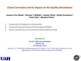
Cloud fraction at 09 CST August 31, 2006 Cloud fraction from MM5 E04 E12 Clear sky on August 31 2006 In E04 domain, model generated too much clouds associated with the low-pressure system (inherited from coarse domain E12/D36). Cloudiness suppresses the photochemical process of ozone over Dallas area. What can we do with wrong cloud & precipitation forecasting???? Test with satellite-obs clouds to modulate J-value Difference plot of O3at11 CST on 8/31 2006 CMAQ run with cloud from MM5 – GOES satellite Observed Cloud fraction E04 Cloud fraction from GOES satellite prepared by University of Alabama, Huntsville (UAH)
Precipitation Event on 8/23 Radar Image 1-hr Precip. from MM5 (shaded) & CMAS observation (circle) at 13 CST on August 23, 2006 Dallas Houston O3 spatial plot at 15 CST on August 23, 2006 Over-prediction of O3 due to inaccurate precipitation simulation from MM5.
Cloud fraction at 12 CST on August 23, 2006 Observed Cloud fraction from GOES satellite (UAH) Cloud fraction from MM5 Difference plot of O3at15 CST on Aug. 23rd 2006 CMAQ run with cloud from MM5 – GOES satellite Ozone difference can be easily ~ 20 ppb!
IC Example Northwest Deer Park AQF AQF Clean IC Clean IC Galveston Bayland AQF AQF Clean IC Clean IC
IC Example Northwest Deer Park AQF AQF Clean IC Clean IC Galveston Bayland AQF AQF IC for August 24 was too high due to missed Precipitation events in the met simulations. Fixing IC corrects overprediction problems Clean IC Clean IC
So many things can go wrong leading to bad air quality forecasting Investigation of causes of bad forecasting may lead to future improvements First, look at the impact of meteorological forecasting (winds, clouds, precipitation, temperature, humidity …) If met forecasting was quite wrong previous day, consider “reinitializing” before next forecasting (not easy!) Uncertainty in emissions need to be improved but most likely for next forecasting season Need to prepare for real-time data assimilation tools, methods, and data (e.g., intermittent emissions from forest fire, volcanic ashes, long-range transport) Continued improvement of model algorithms Conclusive Remarks