Download
1 / 87
870 likes | 904 Views
Explore different search strategies in artificial intelligence, including uninformed techniques like breadth-first and depth-first, and informed techniques like best-first and A* search.

E N D
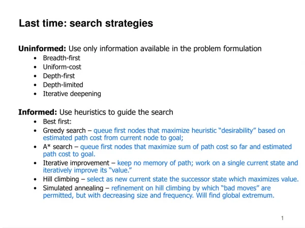
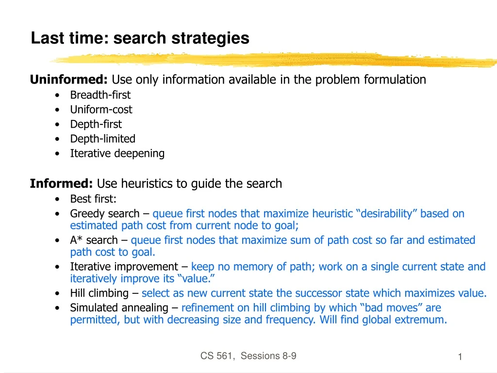
Last time: search strategies Uninformed: Use only information available in the problem formulation • Breadth-first • Uniform-cost • Depth-first • Depth-limited • Iterative deepening Informed: Use heuristics to guide the search • Best first: • Greedy search – queue first nodes that maximize heuristic “desirability” based on estimated path cost from current node to goal; • A* search – queue first nodes that maximize sum of path cost so far and estimated path cost to goal. • Iterative improvement – keep no memory of path; work on a single current state and iteratively improve its “value.” • Hill climbing – select as new current state the successor state which maximizes value. • Simulated annealing – refinement on hill climbing by which “bad moves” are permitted, but with decreasing size and frequency. Will find global extremum. CS 561, Sessions 8-9
A 3 5 B 19 C D 6 h=18 h=15 5 5 4 H E F G h=10 h=12 h=8 h=10 Exercise: Search Algorithms The following figure shows a portion of a partially expanded search tree. Each arc between nodes is labeled with the cost of the corresponding operator, and the leaves are labeled with the value of the heuristic function, h. Which node (use the node’s letter) will be expanded next by each of the following search algorithms? (a)Depth-first search (b)Breadth-first search (c)Uniform-cost search (d)Greedy search (e) A* search h=20 h=14 CS 561, Sessions 8-9
Depth-first search Node queue: initialization # state depth path cost parent # 1 A 0 0 -- CS 561, Sessions 8-9
Depth-first search Node queue: add successors to queue front; empty queue from top # state depth path cost parent # 2 B 1 3 1 3 C 1 19 1 4 D 1 5 1 1 A 0 0 -- CS 561, Sessions 8-9
Depth-first search Node queue: add successors to queue front; empty queue from top # state depth path cost parent # 5 E 2 7 2 6 F 2 8 2 7 G 2 8 2 8 H 2 9 2 2 B 1 3 1 3 C 1 19 1 4 D 1 5 1 1 A 0 0 -- CS 561, Sessions 8-9
Depth-first search Node queue: add successors to queue front; empty queue from top # state depth path cost parent # 5 E 2 7 2 6 F 2 8 2 7 G 2 8 2 8 H 2 9 2 2 B 1 3 1 3 C 1 19 1 4 D 1 5 1 1 A 0 0 -- CS 561, Sessions 8-9
A 3 5 B 19 C D 6 h=18 h=15 5 5 4 H E F G h=10 h=12 h=8 h=10 Exercise: Search Algorithms The following figure shows a portion of a partially expanded search tree. Each arc between nodes is labeled with the cost of the corresponding operator, and the leaves are labeled with the value of the heuristic function, h. Which node (use the node’s letter) will be expanded next by each of the following search algorithms? (a)Depth-first search (b)Breadth-first search (c)Uniform-cost search (d)Greedy search (e) A* search h=20 h=14 CS 561, Sessions 8-9
Breadth-first search Node queue: initialization # state depth path cost parent # 1 A 0 0 -- CS 561, Sessions 8-9
Breadth-first search Node queue: add successors to queue end; empty queue from top # state depth path cost parent # 1 A 0 0 -- 2 B 1 3 1 3 C 1 19 1 4 D 1 5 1 CS 561, Sessions 8-9
Breadth-first search Node queue: add successors to queue end; empty queue from top # state depth path cost parent # 1 A 0 0 -- 2 B 1 3 1 3 C 1 19 1 4 D 1 5 1 5 E 2 7 2 6 F 2 8 2 7 G 2 8 2 8 H 2 9 2 CS 561, Sessions 8-9
Breadth-first search Node queue: add successors to queue end; empty queue from top # state depth path cost parent # 1 A 0 0 -- 2 B 1 3 1 3 C 1 19 1 4 D 1 5 1 5 E 2 7 2 6 F 2 8 2 7 G 2 8 2 8 H 2 9 2 CS 561, Sessions 8-9
A 3 5 B 19 C D 6 h=18 h=15 5 5 4 H E F G h=10 h=12 h=8 h=10 Exercise: Search Algorithms The following figure shows a portion of a partially expanded search tree. Each arc between nodes is labeled with the cost of the corresponding operator, and the leaves are labeled with the value of the heuristic function, h. Which node (use the node’s letter) will be expanded next by each of the following search algorithms? (a)Depth-first search (b)Breadth-first search (c)Uniform-cost search (d)Greedy search (e) A* search h=20 h=14 CS 561, Sessions 8-9
Uniform-cost search Node queue: initialization # state depth path cost parent # 1 A 0 0 -- CS 561, Sessions 8-9
Uniform-cost search Node queue: add successors to queue so that entire queue is sorted by path cost so far; empty queue from top # state depth path cost parent # 1 A 0 0 -- 2 B 1 3 1 3 D 1 5 1 4 C 1 19 1 CS 561, Sessions 8-9
Uniform-cost search Node queue: add successors to queue so that entire queue is sorted by path cost so far; empty queue from top # state depth path cost parent # 1 A 0 0 -- 2 B 1 3 1 3 D 1 5 1 5 E 2 7 2 6 F 2 8 2 7 G 2 8 2 8 H 2 9 2 4 C 1 19 1 CS 561, Sessions 8-9
Uniform-cost search Node queue: add successors to queue so that entire queue is sorted by path cost so far; empty queue from top # state depth path cost parent # 1 A 0 0 -- 2 B 1 3 1 3 D 1 5 1 5 E 2 7 2 6 F 2 8 2 7 G 2 8 2 8 H 2 9 2 4 C 1 19 1 CS 561, Sessions 8-9
A 3 5 B 19 C D 6 h=18 h=15 5 5 4 H E F G h=10 h=12 h=8 h=10 Exercise: Search Algorithms The following figure shows a portion of a partially expanded search tree. Each arc between nodes is labeled with the cost of the corresponding operator, and the leaves are labeled with the value of the heuristic function, h. Which node (use the node’s letter) will be expanded next by each of the following search algorithms? (a)Depth-first search (b)Breadth-first search (c)Uniform-cost search (d)Greedy search (e) A* search h=20 h=14 CS 561, Sessions 8-9
Greedy search Node queue: initialization # state depth path cost total parent # cost to goal cost 1 A 0 0 20 20 -- CS 561, Sessions 8-9
Sort key Greedy search Node queue: Add successors to queue, sorted by cost to goal. # state depth path cost total parent # cost to goal cost 1 A 0 0 20 20 -- 2 B 1 3 14 17 1 3 D 1 5 15 20 1 4 C 1 19 18 37 1 CS 561, Sessions 8-9
Greedy search Node queue: Add successors to queue, sorted by cost to goal. # state depth path cost total parent # cost to goal cost 1 A 0 0 20 20 -- 2 B 1 3 14 17 1 5 G 2 8 8 16 2 7 E 2 7 10 17 2 6 H 2 9 10 19 2 8 F 2 8 12 20 2 3 D 1 5 15 20 1 4 C 1 19 18 37 1 CS 561, Sessions 8-9
Greedy search Node queue: Add successors to queue, sorted by cost to goal. # state depth path cost total parent # cost to goal cost 1 A 0 0 20 20 -- 2 B 1 3 14 17 1 5 G 2 8 8 16 2 7 E 2 7 10 17 2 6 H 2 9 10 19 2 8 F 2 8 12 20 2 3 D 1 5 15 20 1 4 C 1 19 18 37 1 CS 561, Sessions 8-9
A 3 5 B 19 C D 6 h=18 h=15 5 5 4 H E F G h=10 h=12 h=8 h=10 Exercise: Search Algorithms The following figure shows a portion of a partially expanded search tree. Each arc between nodes is labeled with the cost of the corresponding operator, and the leaves are labeled with the value of the heuristic function, h. Which node (use the node’s letter) will be expanded next by each of the following search algorithms? (a)Depth-first search (b)Breadth-first search (c)Uniform-cost search (d)Greedy search (e) A* search h=20 h=14 CS 561, Sessions 8-9
A* search Node queue: initialization # state depth path cost total parent # cost to goal cost 1 A 0 0 20 20 -- CS 561, Sessions 8-9
Sort key A* search Node queue: Add successors to queue, sorted by total cost. # state depth path cost total parent # cost to goal cost 1 A 0 0 20 20 -- 2 B 1 3 14 17 1 3 D 1 5 15 20 1 4 C 1 19 18 37 1 CS 561, Sessions 8-9
A* search Node queue: Add successors to queue front, sorted by total cost. # state depth path cost total parent # cost to goal cost 1 A 0 0 20 20 -- 2 B 1 3 14 17 1 5 G 2 8 8 16 2 6 E 2 7 10 17 2 7 H 2 9 10 19 2 3 D 1 5 15 20 1 8 F 2 8 12 20 2 4 C 1 19 18 37 1 CS 561, Sessions 8-9
A* search Node queue: Add successors to queue front, sorted by total cost. # state depth path cost total parent # cost to goal cost 1 A 0 0 20 20 -- 2 B 1 3 14 17 1 5 G 2 8 8 16 2 6 E 2 7 10 17 2 7 H 2 9 10 19 2 3 D 1 5 15 20 1 8 F 2 8 12 20 2 4 C 1 19 18 37 1 CS 561, Sessions 8-9
A 3 5 B 19 C D 6 h=18 h=15 5 5 4 H E F G h=10 h=12 h=8 h=10 Exercise: Search Algorithms The following figure shows a portion of a partially expanded search tree. Each arc between nodes is labeled with the cost of the corresponding operator, and the leaves are labeled with the value of the heuristic function, h. Which node (use the node’s letter) will be expanded next by each of the following search algorithms? (a)Depth-first search (b)Breadth-first search (c)Uniform-cost search (d)Greedy search (e) A* search h=20 h=14 CS 561, Sessions 8-9
Last time: Simulated annealing algorithm • Idea: Escape local extrema by allowing “bad moves,” but gradually decrease their size and frequency. Note: goal here is to maximize E. - CS 561, Sessions 8-9
Last time: Simulated annealing algorithm • Idea: Escape local extrema by allowing “bad moves,” but gradually decrease their size and frequency. Algorithm when goal is to minimize E. - < - CS 561, Sessions 8-9
This time: Outline • Game playing • The minimax algorithm • Resource limitations • alpha-beta pruning • Elements of chance CS 561, Sessions 8-9
What kind of games? • Abstraction: To describe a game we must capture every relevant aspect of the game. Such as: • Chess • Tic-tac-toe • … • Accessibleenvironments: Such games are characterized by perfect information • Search: game-playing then consists of a search through possible game positions • Unpredictable opponent: introduces uncertainty thus game-playing must deal with contingency problems CS 561, Sessions 8-9
Searching for the next move • Complexity: many games have a huge search space • Chess: b = 35, m=100 nodes =35 100if each node takes about 1 ns to explore then each move will take about 10 50 millenniato calculate. • Resource (e.g., time, memory) limit: optimal solution not feasible/possible, thus must approximate • Pruning: makes the search more efficient by discarding portions of the search tree that cannot improve quality result. • Evaluation functions:heuristics to evaluate utility of a state without exhaustive search. CS 561, Sessions 8-9
Two-player games • A game formulated as a search problem: • Initial state: ? • Operators: ? • Terminal state: ? • Utility function: ? CS 561, Sessions 8-9
Two-player games • A game formulated as a search problem: • Initial state: board position and turn • Operators: definition of legal moves • Terminal state: conditions for when game is over • Utility function: a numeric value that describes the outcome of the game. E.g., -1, 0, 1 for loss, draw, win. (AKA payoff function) CS 561, Sessions 8-9
Game vs. search problem CS 561, Sessions 8-9
Example: Tic-Tac-Toe CS 561, Sessions 8-9
Type of games CS 561, Sessions 8-9
Type of games CS 561, Sessions 8-9
The minimax algorithm • Perfect play for deterministic environments with perfect information • Basic idea: choose move with highest minimax value = best achievable payoff against best play • Algorithm: • Generate game tree completely • Determine utility of each terminal state • Propagate the utility values upward in the three by applying MIN and MAX operators on the nodes in the current level • At the root node use minimax decision to select the move with the max (of the min) utility value • Steps 2 and 3 in the algorithm assume that the opponent will play perfectly. CS 561, Sessions 8-9
Generate Game Tree CS 561, Sessions 8-9
Generate Game Tree CS 561, Sessions 8-9
Generate Game Tree CS 561, Sessions 8-9
Generate Game Tree 1 ply 1 move CS 561, Sessions 8-9
x x x x x x x x x x x x x x x x x x x x x x x x x x o o o o o o o o o o o o o o o o o o o o o o o o o o o o x x x x x x x x x x x x x x o o o o o o o o o o o o o o x x x x x x x A subtree win lose draw x o o o x x o o o x x o x o x o x x x x o x CS 561, Sessions 8-9
x x x x x x x x x x x x x x x x x x x x x x x x x x o o o o o o o o o o o o o o o o o o o o o o o o o o o o x x x x x x x x x x x x x x o o o o o o o o o o o o o o x x x x x x x What is a good move? win lose draw x o o o x x o o o x x o x o x o x x x x o x CS 561, Sessions 8-9
Minimax 3 12 8 2 4 6 14 5 2 • Minimize opponent’s chance • Maximize your chance CS 561, Sessions 8-9
Minimax 3 2 2 MIN 3 12 8 2 4 6 14 5 2 • Minimize opponent’s chance • Maximize your chance CS 561, Sessions 8-9
Minimax 3 MAX 3 2 2 MIN 3 12 8 2 4 6 14 5 2 • Minimize opponent’s chance • Maximize your chance CS 561, Sessions 8-9
Minimax 3 MAX 3 2 2 MIN 3 12 8 2 4 6 14 5 2 • Minimize opponent’s chance • Maximize your chance CS 561, Sessions 8-9
minimax = maximum of the minimum 1st ply 2nd ply CS 561, Sessions 8-9