Download
1 / 68
680 likes | 788 Views
Gradient Networks. (a random tutorial). With:. M. Anghel (LANL), K.E. Bassler (Houston), G. Korniss (RPI), B. Kozma (Paris-Sud), E. Ravasz-Reagan (Harvard), A. Clauset (SFI), E. Lopez (LANL), C. Moore (UNM/SFI). zoltán toroczkai. Physics Department, University of Notre Dame.

E N D
Gradient Networks (a random tutorial) With: M. Anghel (LANL), K.E. Bassler (Houston), G. Korniss (RPI), B. Kozma (Paris-Sud), E. Ravasz-Reagan (Harvard), A. Clauset (SFI), E. Lopez (LANL), C. Moore (UNM/SFI). zoltán toroczkai Physics Department, University of Notre Dame
What are Agent-based Systems? We are rather familiar with: Classical physical, chemical, and certain biological systems: • Elementary particles, nuclei, atoms, molecules, proteins, polymers, fluids, solids, etc. • They are single- or many-particle systems with well defined physical interactions. • Their properties and behavior are well described by the known laws of physics and chemistry. • These properties (including the statistical ones) are reproducible. There are, however, other types of ubiquitous systems surrounding us: Agent-based Systems.
Social Insects Collective behavior from simple individuals. High level of organization forming “social structures (hierarchies). The individual usually cannot exist/survive on its own.
For efficient foraging, memory of locations is needed. Memory is introduced via pheromone trails. This is a “collective memory” !
Humans As a collective they too, can form low-entropy formations:
Or, high entropy formations, or crowds: while having fun … …or just plain panicked
… markets… in New York … or middle-east … and economies:
Let us attempt a unifying representation: ABS-s are systems of interacting entities called agents / players / individuals. An agent is an entity with the following set of qualities: • There is a set of variables x describing the state of the agent. (position, speed, health state, etc.). The corresponding state space is X. • There is a set of variables z, describing the perceived state of the environment, Z. The environment includes other agents if there are any. • There is a set of allowable actions (output space), A. (swerve, brake, accelerate, etc.) • There is a set of strategies, which are functions s: (ZX)t A, that summon an action to a given external perception, state of the agent and history up to time t. These are “ways of thinking” for the agent. Behavioral input space. • There is a set of utility variables, uU. (time to destination, profits, risk) • There is a multivariate objective function: F:URm, which might include constraints (“rules”). The physics version is called action. • There is adrive to optimize the objective function. The topologyof the interactionsis usually a dynamical graph, or network.
Agent-based systems are really nothing more than a set of coupled optimizers. Problem Classes • The “Forward” or Analysisproblem: mapping out collective behavior from the study of interactions on the individual level (from micro to macro approach). • The “Backward” or Design problem: there is an additional set of global variables that form the utility space of the designer. Define individual traits and response functions such that a global optimal performance is induced.
Would Statistical Physics like methods work? Deductive Game Theory Classical Statistical Mechanics (von Neumann and Morgenstern ) • single response function (Hamiltonian) - rational behavior - algorithmic choice tree evaluation - non-adaptive - large particle limit N ~ 1023 - agent-planning Agent-based Systems • multiple response fcts. explosion of state space - adaptive - individual goal-driven (coupled set of optimizers) - mesoscopic size N ~ 108 - bounded rationality behavior (“good news”) (Brian W. Arthur, 1994) - broad distribution of interaction scales
Approaches of study: Stylized (theoretical): build models from ingredients that qualitatively match observations. After running the model see if the output qualitatively matches the corresponding observations of the real system. Gives a general understanding only, no quantitative predictive capability. Bottom-up (simulation and data heavy): insert as much quantitative detail as possible along with real-world data. Run the model over and over with different data. Perform statistics and compare results with statistics measured on the real system. Some predictive capability. Industry, government. Icosystems, Eric Bonabeau
The following slides represent example of a stylized model of a market. This is an agent-based system where we study the qualitative behavior of a collective of interacting agents under certain conditions, in particular that of limited resources. It lead us to the introduction of the notion of gradient networks. Competition Games on Networks • Marian Anghel (LANL) • Kevin E. Bassler (U. Houston) • György Korniss (Rensselaer) Collaboration with: References: M. Anghel, Z. Toroczkai, K.E. Bassler and G. Korniss, Competition-driven Network Dynamics: Emergence of a Scale-free Leadership Structure and Collective Efficiency, Phys.Rev.Lett.92, 058701 (2004) Z. Toroczkai, M. Anghel, G. Korniss and K.W. Bassler, Effects of Inter-agent Communications on the Collective, in Collectives and the Design of Complex Systems, eds. K. Tumer and D.H. Wolpert, Springer, 2004.
Resource limitations lead in human, and most biological populations to competitive dynamics. The more severe the limitations, the more fierce the competition. Amid competitive conditions certain agents may have better venues or strategies to reach the resources, which puts them into a distinguished class of the “few”, the gurus (elites). They form a minority group. In spite of the minority character, they can considerably shape the structure of the whole society: since they are the most successful (in the given situation), the rest of the agents will tend to follow (imitate, interact with) the gurus creating a social structure of leadership in the agent society. Definition: a leader is an agent that has at least one follower at that moment. The influence of a leader is measured by the number of followers it has. Leaders can be following other leaders or themselves. The non-leaders are coined “followers”.
The El Farol bar problem [W. B Arthur(1994)] A B …
A binary (computer friendly) version of the El Farol bar problem: The Minority Game (MG) [Challet and Zhang (1997)] A = “0” (bar ok, go to the bar) B = “1” (bar crowded, stay home) latest bit l {0,1,..,2m-1} World utility(history): (011..101) m bits S(i)1(l) S(i)2(l) (Strategies)(i) = (Scores)(i) = C (i)(k), k = 1,2,..,S. S(i)S(l) (Prediction) (i) =
A(t) t
Attendance time-series for the MG: World Utility Function: Agents cooperate if they manage to produce fluctuations below (N1/2)/2 (RCG).
The Minority Game on Networks (MGoN) Agents communicate among themselves. Social network: 2 components: 1) Aquintance (substrate) network: G (non-directed, less dynamic) 2) Action network: A (directed and dynamic) G A G A
Emergence of scale-free leadership structure: m=6 • Robust leadership hierarchy • RCG on the ER network produces the scale-free backbone of the leadership structure • The influence is evenly distributed among all levels of the leadership hierarchy.
The followers make up most of the population (over 90%) and their number scales linearly with the total number of agents. • Structural un-evenness appears in the leadership structure for low trait diversity.
Network Effects: Improved Market Efficiency • A networked, low trait diversity system is more effective as a collective than a sophisticated group! • Can we find/evolve networks/strategies that achieve almost perfect volatility given a group and their strategies (or the social network on the group)?
What are networks ? Collection of discrete entities [nodes], which might be connected via links [edges] representing interactions or associations between the connected elements. Mathematical term for these objects: Graph Typical notation: G(V, E), where V={1,2,…,N} is the set of nodes (vertices, sites) and E is theset of edges. An edge typically connects a pair of vertices x and y, however it can also connect more than two vertices, called hyperedges and this case the resulting graph is called a Hypergraph. For now we exclusively deal with simple graphs, where Typical notations for an edge :
If there are several edges between two nodes, the graph is called a multigraph. If the interaction or association is unidirectional, then this fact is resolved by making Such an edge is called a directed edge and the corresponding graph a directed graph, or digraph for short. Note: Both nodes and edges can have associated a number of properties, parameters, called weights. Graphs and weights can be time dependent. Typical real-world graphs are the result of complex processes with stochastic components makes sense to talk about Graph Ensembles and probabilistic descriptions.
Representations: Visual, geometric: Abstract: - e.g. with the adjacency matrix: where • “expensive” representation, requires O(N2) resources • it is hard to simply recover patterns/clusters from. • sometimes advantageous for analytical calculations Finding clusters in networks: “community” detection.
More economical representations: adjacencylists. - standard representation used in algorithmic computations. • Reading: • R. Sedgewick, “Algorithms in (C++), Part 5, Graph Algorithms”, Addison-Wesley, (2002). • Cormen et.al., “Introduction to Algorithms”, The MIT Press, (2001) List Heads Neighbors
Where are Networks? • Infrastructures: transportation nw-s (airports, highways, roads, rail, water) energy transport nw-s (electric power, petroleum, natural gas) • Communications:telephone, microwave backbone, internet, email, www, etc. • Biology:protein-gene interactions, protein-protein interactions, metabolic nw-s, cell-signaling nw-s, the food web, etc. • Social Systems:acquaintance (friendship) nw-s, terrorist nw-s, collaboration networks, epidemic networks, the sex-web • Geology:river networks
Skitter data depicting a macroscopic snapshot of Internet connectivity, with selected backbone ISPs (Internet Service Provider) colored separately by K. C. Claffy email:kc@caida.orghttp://www.caida.org/Papers/Nae/
Biological Networks R.J. Williams, N.D. Martinez Nature (2000) Food Webs trophic species trophic interactions
Cellular Networks: The Bio-Map Source: Barabasi et.al. GENOME Protein-gene interactions PROTEOME Protein-Protein interactions METABOLISM Bio-chemical reactions Citrate Cycle
Metabolic Networks Chemicals Bio-Chemical reactions
Prot P(k) The protein network proteins Binding H. Jeong, S.P. Mason, A.-L. Barabasi, Z.N. Oltvai, Nature411, 41 (2001) P. Uetz, et al.Nature403, 623-7 (2000).
Social Networks person Social interaction, relation (friendship, etc.) Acquaintance networks The sex-web Actor Networks Collaboration Networks person common paper More on social networks later… (Newman, 2000, H. Jeong et al 2001)
How do we describe and study networks? The party problem What is the minimum nr. of people R, one should invite to a party that would surely have k people who all know each other, or k who do not know each other (at all)? For k=3, R(k) =6 Know each other Do not now each other For k=4: R(k) =18 (hard proof)
For k=5: R(k)=… NOT KNOWN! Only the bounds are known: 43 R(5) 49 . Come on, use a computer! We are looking for complete graphs with n nodes that have a monochromatic complete subgraph of k nodes (k-clique). (Here k=5.) There are edges in a complete graph. There are such graphs whose edges are either blue or red. Since for k=3, R(3)=6, an n=6 node complete graph would have a monochromatic triangle. n=6: n=18: graphs. 43 n 49:
Operating at the physical limits of computation (as determined by the Planck constant, the speed of light and the gravitational constant) the 1kg laptop of Set Lloyd performs S. Lloyd, “Ultimate Physical Limits to Computation”, Nature, 406, 1047 (2000). To check all graphs for monochromatic complete subgraphs takes at least Or, for k=5 it would take at least The age of the universe is estimated to be: 1.1-2 1010 yrs! Probabilistic ensemble approach.
Structural properties: degree distributions and the scale-free character Node degree: number of neighbors ki=5 i Degree distribution, P(k):fraction of nodes whose degree is k (a histogram over the ki –s.) Observation: networks found in Nature and human made, are in many cases “scale-free” (power-law) networks:
For the sake of definitions: The Erdős-Rényi Random Graph (also called the binomial random graph) • Consider N nodes (dots). • Take every pair (i,j) of nodes and connect them with an edge with probability p.
The Erdős-Rényi random graph (continued) GN,p is a graph with N vertices and link-probabilityp (the probability that two arbitrarily chosen vertices are connected by an edge). Average nr. of links incident on a node: . Clustering coefficient . The probability of a node having exactly k incident edges is: If Xkdenotes the number of nodes in an instance ofGN,p with degree k, its distribution is not given exactly by P(k)! -- correlations induced by the fact that and edge is shared by two nodes. It is however asymptotically correct (Bollobás). In the limit of N and p0 such that =pN=const. : (Poisson) and Since the width is: the Binomial Random Graph has a characteristic scale given by Can graphs with the same P(k) be very different?
A Very likely! B C ki=5 ni=3 Ci=0.3 i Other graph measures: Clustering or transitivity Clustering distribution: Average clustering coefficient:
Random Geometric Graphs 0 < R 1 Continuum percolation Average degree: Degree distribution is Poisson Clustering coefficient J.Dall, M. Christensen, PRE66, 016121 (2002)
What is scale-free? Poisson distribution Power-law distribution =<k> Erdős-Rényi Graph Capacity achieving degree distribution of Tornado code. The decay exponent -2.02. Non-Scale-free Network M. Luby, M. Mitzenmacher, M.A. Shokrollahi, D. Spielman and V. Stemann, in Proc. 29th ACM Symp. Theor. Comp. pg. 150 (1997). Scale-free Network
Science citations www, out- and in- link distributions Internet, router level Archaea Bacteria Eukaryotes Bacteria Eukaryotes Metabolic network Sex-web
Scale-free Networks: Coincidence or Universality? • No obvious universal mechanism identified • As a matter of fact we claim that there is none (universal that is). • Instead, our statement is that at least for a large class of networks (to be specified) network structural evolution is governed by a selection principle which is closely tied to the global efficiency of transport and flow processing by these structures, and • Whatever the specific mechanism, it is such as to obey this selection principle. Need to define first a flow process on these networks. Z. Toroczkai and K.E. Bassler, “Jamming is Limited in Scale-free Networks”, Nature, 428, 716 (2004) Z. Toroczkai, B. Kozma, K.E. Bassler, N.W. Hengartner and G. Korniss “Gradient Networks”, http://www.arxiv.org/cond-mat/0408262
Gradient Networks Gradients of a scalar (temperature, concentration, potential, etc.) induce flows (heat, particles, currents, etc.). Naturally, gradients will induce flows on networks as well. Ex.: Load balancing in parallel computation and packet routing on the internet Y. Rabani, A. Sinclair and R. Wanka, Proc. 39th Symp. On Foundations of Computer Science (FOCS), 1998:“Local Divergence of Markov Chains and the Analysis of Iterative Load-balancing Schemes”
Setup: Let G=G(V,E) be an undirected graph, which we call the substrate network. The vertex set: The edge set: A simple representation of E is via the Nx N adjacency (or incidence) matrix A (1) Let us consider a scalar field Set of nearest neighbor nodes on G of i :
Definition 1 The gradient h(i) of the field {h} in node i is a directed edge: (2) Which points from i to that nearest neighbor for G for which the increase in the scalar is the largest, i.e.,: (3) The weight associated with edge (i,) is given by: . . The self-loop is a loop through i with zero weight. Definition 2 The set F of directed gradient edges on G together with the vertex set V forms the gradient network: If (3) admits more than one solution, than the gradient in i is degenerate.