Download
1 / 25
300 likes | 586 Views
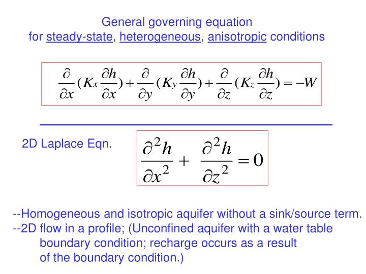
2D Laplace Eqn. --Homogeneous and isotropic aquifer without a sink/source term. --2D flow in a profile; (Unconfined aquifer with a water table boundary condition; recharge occurs as a result of the boundary condition.). General governing equation

E N D
2D Laplace Eqn. --Homogeneous and isotropic aquifer without a sink/source term. --2D flow in a profile; (Unconfined aquifer with a water table boundary condition; recharge occurs as a result of the boundary condition.) General governing equation for steady-state, heterogeneous, anisotropic conditions
Mathematical Model of the Toth Problem Unconfined aquifer h = c x + zo
Aquifer b z x x z b z x Toth problem b = 1 m
Aquifer b 2D horizontal flow in an aquifer with constant thickness, b. y x
unconfined aquifer b is not constant b confined aquifer Figure from Hornberger et al. 1998
Aquifer b 2D horizontal flow in an aquifer with constant thickness, b. with recharge y x
2D horizontal flow 2D horizontal flow; homogeneous and isotropic aquifer with constant aquifer thickness, b, so that T=Kb. with a source/sink term Poisson Equation
South Fork Map of Long Island, N.Y. Charles Edward Jacob (1914-1970) Consultant to the Town of Southampton, NY December 1968
h datum C.E. Jacob’s Conceptual Model of the South Fork of Long Island water table R groundwater divide ocean ocean b x = - L x = 0 x = L We can simulate this system assuming horizontal flow in a “confined” aquifer if we assume that T= Kb.
at x =0 h(L) = 0 1D approximation used by C.E. Jacob R ocean ocean x = - L x = 0 x = L Boundary Conditions Governing Eqn.
C.E. Jacob’s Model Governing Eqn. at x =0 Boundary conditions h(L) = 0 Analytical solution for 1D “confined” version of the problem h(x) = R (L2 – x2) / 2T Forward solution R = (2 T) h(x) / ( L2 – x2) Inverse solution for R
Inverse solution for R R = (2 T) h(x) / ( L2 – x2) Solve for R with h(x) = h(0) = 20 ft. Inverse solution for T Rearrange eqn to solve for T, given value for R and h(0) = 20 ft. Observation well on the groundwater divide L
Island Recharge Problem L y 2L ocean ocean well T= 10,000 ft2/day L = 12,000 ft x ocean
Targets used in Model Calibration • Head measured in an observation well is known as a head target. • The simulated head at the node representing the observation well is compared with the measured head. • During model calibration, parameter values (e.g., R and T) are adjusted until the simulated head matches the observed value. • Model calibration solves the inverse problem.
Island Recharge Problem L = 12,000 ft y 2L ocean Solve the forward problem: Given R= 0.00305 ft/d T= 10,000 ft2/day Solve for h at each nodal point ocean well x ocean
Write the finite difference approximation: Gauss-Seidel Iteration Formula for 2D Poisson Equation with x = y = a
Island Recharge Problem 4 X 7 Grid
Water Balance IN = Out IN = R x AREA Out = outflow to the ocean
Top 4 rows Head at a node is the average head in the area surrounding the node. Red dots represent specified head cells, which are treated as inactive nodes. Black dots are active nodes. (Note that the nodes along the groundwater divides are active nodes.)
L 2L Top 4 rows IN =R x Area = R (L-x/2) (2L - y/2) Also: IN = R (2.5)(5.5)(a2)
x x/2 x Top 4 rows
Qy = (Th) /2 Qy x/2 Qx Top 4 rows OUT = Qy + Qx Qy = K (x b) (h/y) Note: x = y Qy = T h Qx = K (y b)(h/x) or Qx = T h y
Bottom 4 rows y/2 Well Qx = (T h)/2
Island Recharge Problem 4 X 7 Grid