Download

1 / 36
360 likes | 507 Views
Summary Measures of Ungrouped Numerical Data. Comparing Data Sets with respect to:. Location. Variability. (Dispersion). Shape. Calculation and Properties of Some Measures of Variability of Ungrouped Numerical Data. Find the following measures of VARIABILITY (DISPERSION).

E N D
Summary Measures of Ungrouped Numerical Data
Comparing Data Sets with respect to: Location Variability (Dispersion) Shape
Calculation and Properties of Some Measures of Variability of Ungrouped Numerical Data
Find the following measures of VARIABILITY (DISPERSION). 1) Range 2) Interquartile Range (IQR) 3) Variation (SS) 4) Variance (S2) 5) Standard Deviation (S) 6) Coefficient of Variation (CV) First, the range.
Calculation of the Range The following sample (n = 7) of data contains the number of years that a company was in business. For the small sample (n = 7), the range will be calculated. Range = maximum - minimum
Properties of the Range The following sample (n = 7) of data contains the number of years that a company was in business. For this small sample (n = 7), range = 12. The range is a measure of variability (dispersion). It tells how “wide” the values in the data set are spread. Next, a LARGE sample is considered.
A Large Sample Example (presented as Raw Data) The following sample (n = 120) of data contains the number of years that a company was in business. Q: What does one need to know to find the range of the sample above? A: The maximum value and the minimum value. (These are easier to find in the ordered array.)
A Large Sample Example (presented as an Ordered Array) The following sample (n = 120) of data contains the number of years that a company was in business.
Find the following measures of VARIABILITY (DISPERSION). 1) Range 2) Interquartile Range (IQR) 3) Variation (SS) 4) Variance (S2) 5) Standard Deviation (S) 6) Coefficient of Variation (CV) Next, the interquartile range.
Calculation of the Interquartile Range The following sample (n = 7) of data contains the number of years that a company was in business. For the small sample (n = 7), the interquartile range will be calculated. IQR = Interquartile Range = Q3 – Q1 By the formula Q3 = 14 and Q1 = 3 and the IQR = 11. WHY?
Properties of the Interquartile Range The following sample (n = 7) of data contains the number of years that a company was in business. For this small sample (n = 7), IQR = 11. The interquartile range tells how “wide” the values in the data set are spread between the first and the third quartiles. Because ¼ of the data values are ≤ Q1 and ¼ of the data values are ≥ Q3, the middle ½ (or 50%) of the data values are between Q1 and Q3. The IQR is the “spread” of the middle 50% of the data values. Next, a LARGE sample is considered.
A Large Sample Example (presented as Raw Data) The following sample (n = 120) of data contains the number of years that a company was in business. Q: What does one need to know to find the IQR of the sample above? A: The values of the first and the third quartiles. (See the next two slides for finding those two values.) IQR = 15 – 4 = 11
A Large Sample Example (presented as an Ordered Array) The following sample (n = 120) of data contains the number of years that a company was in business. Position 30. Position 31. The position is closer to 30 than 31, so the value of Q1 is the value at position 30.
A Large Sample Example (presented as an Ordered Array) The following sample (n = 120) of data contains the number of years that a company was in business. Position 90. Position 91. The position is closer to 91 than 90, so the value of Q3 is the value at position 91.
Find the following measures of VARIABILITY (DISPERSION). 1) Range 2) Interquartile Range (IQR) 3) Variation (SS) 4) Variance (S2) 5) Standard Deviation (S) 6) Coefficient of Variation (CV) } The next three measures will be treated as a set of three steps.
A Large Sample Example (presented as Raw Data) The following sample (n = 120) of data contains the number of years that a company was in business. Remember the question below. The answer comes in step 3. The answer is called the standard deviation. If , then what is the “typical” number of years that a value in the sample differs from the mean?
Concept of the Standard Deviation The following sample (n = 7) of data contains the number of years that a company was in business. For the small sample (n = 7), the standard deviation will be found. The symbol used for the sample standard deviation is S. The standard deviation of the sample is a value that represents the “typical” deviation from the sample mean. For the small sample above the mean (X-bar) is 9. The deviations from the mean are: (10-9), (6-9), (14-9), (15-9), (3-9), (12-9), and (3-9). For the small sample above the seven deviations from the mean are: (+1), (-3), (+5), (+6), (-6), (+3), and (-6). What is the “typical” deviation from the mean?
Concept of the Standard Deviation The following sample (n = 7) of data contains the number of years that a company was in business. Could the “typical” deviation from the mean be the mean of all the deviations from the mean? The mean of the deviations from the mean is the sum of the deviations from the mean divided by the number of deviations from the mean.
Concept of the Standard Deviation The following sample (n = 7) of data contains the number of years that a company was in business. However, the sum of the deviations from the mean is always ZERO! No matter how far the deviations are from the mean, the negative deviations will balance out the positive deviations in the sum. How can we “measure” the deviations without the positives and negatives “balancing” each other out?
Concept of the Standard Deviation The following sample (n = 7) of data contains the number of years that a company was in business. • There are two common ways for preventing the balancing • of the positive and negative deviations: • Take the absolute value of each deviation and calculate • the mean absolute deviation (the M.A.D. statistic). • Take the square of each deviation; sum them to find the • variation; divide by the degrees of freedom to find the • variance; take the square root to find the standard deviation.
Concept of the Standard Deviation The following sample (n = 7) of data contains the number of years that a company was in business. • In a sense, the M.A.D. statistic represents the “typical” • deviation from the mean. It is simpler to calculate, but • mathematically the absolute value function is not as • “nice” as the square function. (It is not differentiable at zero.) • Thus, the standard deviation is ordinarily used to • represent the “typical” deviation from the mean. • By definition, you can find the standard deviation by: • Calculating each deviation from the mean. • Squaring each of these deviations. • Summing the squares of the deviations to obtain the variation. • Dividing the variation by (n-1) to obtain the variance. • Taking the square root of the variance.
Calculation of the Standard Deviation The following sample (n = 7) of data contains the number of years that a company was in business. For the small sample (n = 7), the standard deviation will be found. The symbol used for the sample standard deviation is S.
Calculation of the Standard Deviation The following sample (n = 7) of data contains the number of years that a company was in business. For the small sample (n = 7), the standard deviation will be found. The symbol used for the sample standard deviation is S. Next, a LARGE sample is considered.
A Large Sample Example (presented as Raw Data) The following sample (n = 120) of data contains the number of years that a company was in business. Q: What does one need to know to find the standard deviation of the sample above? A: The sum of the values, the sum of the squares of the values, and the sample size (n).
A Large Sample Example (presented as Raw Data) The following sample (n = 120) of data contains the number of years that a company was in business.
Find the following measures of VARIABILITY (DISPERSION). 1) Range 2) Interquartile Range (IQR) 3) Variation (SS) 4) Variance (S2) 5) Standard Deviation (S) 6) Coefficient of Variation (CV) Next, the coefficient of variation.
Concept of the Coefficient of Variation Suppose there are multiple data sets (not just one). How does one determine which data set has the largest amount of variability in it? A logical choice is to use the standard deviation. If data set B has a larger standard deviation than data set A, then B is more variable, right? Consider the following example.
Concept of the Coefficient of Variation Data set A has a standard deviation of approximately 21.6, whereas data set B has a standard deviation of approximately 289.5. Clearly data set B is more variable, RIGHT? Actually the two data sets ARE THE SAME! Data Set A are items priced in US dollars, whereas data set B contains the same items priced in Mexican pesos (13.4 Mexican pesos to the US dollar).
Concept of the Coefficient of Variation Suppose there are multiple data sets (not just one). In many instances the coefficient of variation (usually expressed as a percentage) will allow one to determine which data set has the largest amount of variability in it. Coefficient of Variation (CV)
Concept of the Coefficient of Variation Suppose there are multiple data sets (not just one). In many instances the coefficient of variation (usually expressed as a percentage) will allow one to determine which data set has the largest amount of variability in it. Coefficient of Variation (CV) CV = (standard deviation / mean) X 100
Concept of the Coefficient of Variation Suppose there are multiple data sets (not just one). In many instances the coefficient of variation (usually expressed as a percentage) will allow one to determine which data set has the largest amount of variability in it. Coefficient of Variation (CV) CV = (standard deviation / mean) X 100 The coefficient of variation (usually expressed as a percentage) measures how large the standard deviation is relative to the mean. Consider the previous example.
Concept of the Coefficient of Variation Data set A has a standard deviation of approximately 21.6, whereas data set B has a standard deviation of approximately 289.5. The coefficient of variation yields the same value for both.
Concept of the Coefficient of Variation Data set A has a standard deviation of approximately 21.6, whereas data set B has a standard deviation of approximately 289.5. The coefficient of variation yields the same value for both.
Concept of the Coefficient of Variation See the stock price data in the Excel file, 1-ungrouped.xls, for another example of using the coefficient of variation to determine which data set has the larger variability. Coefficient of Variation (CV) CV = (standard deviation / mean) X 100 Ordinarily, the larger the value of the CV, the more variability there is in the data set.
Concept of the Coefficient of Variation See the stock price data in the Excel file, 1-ungrouped.xls, for another example of using the coefficient of variation to determine which data set has the larger variability. Coefficient of Variation (CV) CV = (standard deviation / mean) X 100 Ordinarily, the larger the value of the CV, the more variability there is in the data set. Next, SHAPE is examined.