Download

1 / 40
400 likes | 654 Views
THE BEHAVIOUR OF PREDATORS. THE BEHAVIOUR OF PREDATORS. The food of Predators is determined by 1. The type of prey – preference (selection) 2. The density of the prey. THE BEHAVIOUR OF PREDATORS. Predators show a PREFERENCE when they select prey:

E N D
THE BEHAVIOUR OF PREDATORS The food of Predators is determined by 1. The type of prey – preference (selection) 2. The density of the prey
THE BEHAVIOUR OF PREDATORS Predators show a PREFERENCE when they select prey: Preference is shown when the proportion of a food type in the diet is higher than the proportion available to the animal
Wagtails select (red) a smaller size of fly than that available (green)
THE BEHAVIOUR OF PREDATORS • Predators show SWITCHING when a prey type is • initially rare then becomes abundant • when rare the predator ignores it • when common the predator shows preference
Predators are selecting if red line is above broken line
THE BEHAVIOUR OF PREDATORS The food of Predators is determined by 2. The density of the prey Animals eat more when there is more available to eat. This is called the FUNCTIONAL RESPONSE. Identified by C.S. (Buzz) Holling 1959 (from UBC). The functional response is the relationship between the amount a single predator eats relative to the density of prey available The simple relationship is a TYPE I
TYPE I FUNCTIONAL RESPONSE – Reindeer eating lichens
SATIATION and HANDLING Reasons for changes in food intake rate 1. There is a finite stomach capacity - satiation 2. There is a finite amount of time in a day to handle prey. Handling time includes: Catching Killing Eating Digesting With high numbers of prey eventually all time is taken up with handling. Results in a curve called the TYPE II FUNCTIONAL RESPONSE
The different types of FUNCTIONAL RESPONSE Density ->
Type II Functional Response of Bay-breasted warblers to outbreaks of spruce budworm larvae – eastern Canada
TYPE II FUNCTIONAL RESPONSE - lynx feeding on snowshoe hares, northern Canada
TYPE II FUNCTIONAL RESPONSE - kestrels feeding on voles Bank voles feeding on shrubs
TYPE III FUNCTIONAL RESPONSE Occurs when the prey is initially rare and the predator ignores it, then switches to eating this prey when it becomes more common. Results in an S-shaped curve
TYPE III FUNCTIONAL RESPONSE – harriers (raptors) feeding on grouse chicks
NUMERICAL RESPONSE Reasons why numbers level off as prey density increases: 1. Searching efficiency declines due to interference between predators – often with insects 2. Territoriality - sequesters space and limits numbers - another form of interference
NUMERICAL RESPONSE – warbler breeding numbers relative to food density
NUMERICAL RESPONSE – wolf numbers relative to moose density, Ontario
TOTAL RESPONSE By multiplying the proportion of prey population killed by each predator (Functional response) and the number of predators we get the total proportion of prey killed by the predator population, called the TOTAL RESPONSE %Total killed by the predator population (TR) = %killed by one predator x number of predators
Total response – mice and shrews feeding on sawfly cocoons (a kind of wasp) Total response – wolves feeding on moose in Ontario
Inverse density dependent predation of small predators on bird nests in forest fragments - eastern forests of USA = Type II FR
% Prey recruitment Total response and prey recruitment - Type II FR C is stable B is unstable Total response = % predation %
TOTAL RESPONSE TYPE II NOTES 1. Occurs when there is a Type II functional response 2. The predator has another food source, the primary prey on which it depends 3. There is no refuge for the prey There can be different levels of predation, with different consequences: Curve i). System stabilizes at C, predator cannot eliminate prey Curve ii) There is a stable point at C, and an unstable threshold at B. If prey numbers are reduced below B for some other reason, then predators can cause extinction of prey Curve iii) Highest level of predation – above the prey recruitment curve at all prey densities. This system cannot exist except as a transition phase to extinction. There are no stable points.
RED FOX – supported by rabbits could eliminate the smaller Marsupials in Australia
MOOSE – spread through BC and support higher populations of wolves
CARIBOU – in BC reduced to extinction by wolves which are maintained by Moose
Caribou in BC forests - r declines faster at small numbers due to Inverse density dependent predation from wolves
Total response and prey recruitment - Type III FR % Prey NET recruitment Total response = % predation % Prey density
TOTAL RESPONSE TYPE III NOTES 1. Occurs when there is a Type III functional response 2. The predator depends on this prey, the primary prey 3. The predator cannot cause extinction because at low prey densities predation is density dependent. There is always a stable point at A There can be different levels of predation, with different consequences: Curve i). System stabilizes at A, predators regulate prey at all prey densities Curve ii) There is a stable point at C, predators eat starving prey. Curve iii) There are two stable points A,C and an unstable boundary B between them. If high prey numbers are below B the system collapses to A. Alternatively if low prey numbers are allowed to increase above B then system outbreaks to C.