Chapter 23 Probabilistic Language Processing

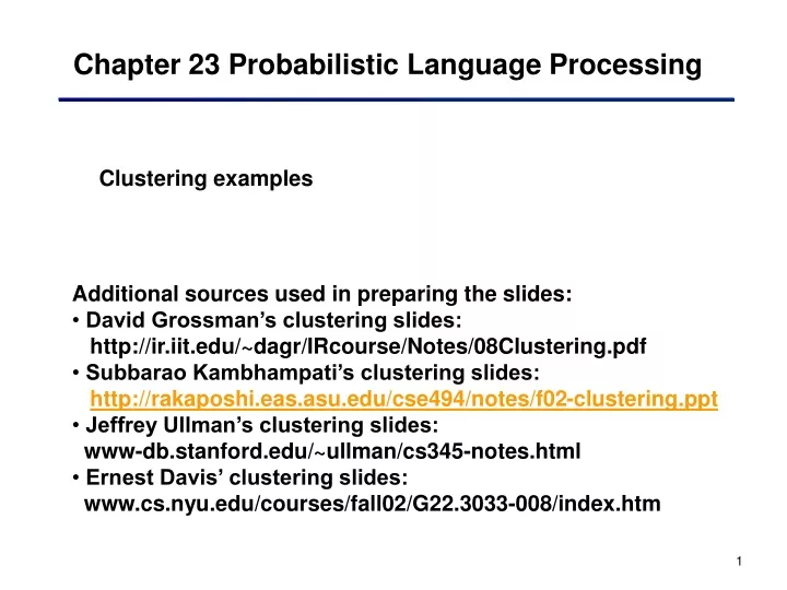
1. Chapter 23 Probabilistic Language Processing • Clustering examples • Additional sources used in preparing the slides: • David Grossman’s clustering slides: http://ir.iit.edu/~dagr/IRcourse/Notes/08Clustering.pdf • Subbarao Kambhampati’s clustering slides:http://rakaposhi.eas.asu.edu/cse494/notes/f02-clustering.ppt • Jeffrey Ullman’s clustering slides: www-db.stanford.edu/~ullman/cs345-notes.html • Ernest Davis’ clustering slides: www.cs.nyu.edu/courses/fall02/G22.3033-008/index.htm

2. Unsupervised learning

3. Example: a cholera outbreak in London • Many years ago, during a cholera outbreak in London, a physician plotted the location of cases on a map. Properly visualized, the data indicated that cases clustered around certain intersections, where there were polluted wells, not only exposing the cause of cholera, but indicating what to do about the problem. X X X X X X X X X X X X X X X X X X X X X

4. Conceptual Clustering • The clustering problem • Given • a collection of unclassified objects, and • a means for measuring the similarity of objects (distance metric), • find • classes (clusters) of objects such that some standard of quality is met (e.g., maximize the similarity of objects in the same class.) • Essentially, it is an approach to discover a useful summary of the data.

5. Conceptual Clustering (cont’d) • Ideally, we would like to represent clusters and their semantic explanations. In other words, we would like to define clusters extensionally (i.e., by general rules) rather than intensionally (i.e., by enumeration). • For instance, compare • { X | X teaches AI at MTU CS}, and • { John Lowther, Nilufer Onder}

6. Curse of dimensionality • While clustering looks intuitive in 2 dimensions, many applications involve 10 or 10,000 dimensions • High-dimensional spaces look different: the probability of random points being close drops quickly as the dimensionality grows

7. Higher dimensional examples • Observation that customers who buy diapers are more likely to buy beer than average allowed supermarkets to place beer and diapers nearby, knowing many customers would walk between them. Placing potato chips between increased the sales of all three items.

8. SkyServer

9. Sloan Digital Sky Survey • A cool tool to “map the universe” • Objects are represented by their radiation in 9 dimensions (each dimension represents radiation in one band of the spectrum) • Clustered 2 x 109 sky objects into similar objects e.g., stars, galaxies, quasars, etc. • The objective was to catalog and cluster the entire visible universe. Clustering sky objects by their radiation levels in different bands allowed astronomers to distinguish between galaxies, nearby stars, and many other kinds of celestial objects.

10. Clustering CDs • Intuition: music divides into categories and customers prefer a few categories • But what are categories really? • Represent a CD by the customers who bought it • Similar CDs have similar sets of customers and vice versa

11. The space of CDs • Think of a space with one dimension for each customer • Values in a dimension may be 0 or 1 only • A CD’s point in this space is (x1, x2, …, xn), where xi = 1 iff the ith customer bought the CD • Compare this with the correlated items matrix:rows = customerscolumns = CDs

12. Clustering documents • Query “salsa” submitted to MetaCrawler returns the following documents among others: • How to dance salsa • Gourmet salsa • Diet seen on Rachael Ray • Michigan Salsa • It also asks: “Are you looking for?” • Music salsa • Salsa recipe • Homemade salsa recipe • Salsa dancing • The clusters are: dance, recipe, clubs, sauces, buy, Mexican, bands, natural, …

13. Clustering documents (cont’d) • Documents may be thought of as points in a high-dimensional space, where each dimension corresponds to one possible word. • Clusters of documents in this space often correspond to groups of documents on the same topic, i.e., documents with similar sets of words may be about the same topic • Represent a document by a vector (x1, x2, …, xn), where xi = 1 iff the ith word (in some order) appears in the document • n can be infinite

14. Analyzing protein sequences • Objects are sequences of {C, A, T, G} • Distance between sequences is “edit distance,” the minimum number of inserts and deletes to turn one into the other • Note that there is a “distance,” but no convenient space of points

15. Measuring distance • To discuss, whether a set of points is close enough to be considered a cluster, we need a distance measureD(x,y) that tells how far points x and y are. • The axioms for a distance measure D are: 1. D(x,x) = 0 A point is distance 0 from itself 2. D(x,y) = D(y,x) Distance is symmetric 3. D(x,y) ≤ D(x,z) + D(z,y) The triangle inequality • 4. D(x,y) ≥ 0Distance is positive

16. K-dimensional Euclidean space • The distance between any two points, saya = [a1, a2, … , ak] and b = [b1, b2, … , bk]is given in some manner such as: • 1. Common distance (“L2 norm”) :i =1 (ai - bi)2 2. Manhattan distance (“L1 norm”): i =1 |ai - bi|3. Max of dimensions (“L norm”): maxi =1 |ai - bi| b k a b k a b k a

17. Non-Euclidean spaces • Here are some examples where a distance measure without a Euclidean space makes sense. • Web pages: Roughly 108-dimensional space where each dimension corresponds to one word. Rather use vectors to deal with only the words actually present in documents a and b. • Character strings, such as DNA sequences: Rather use a metric based on the LCS---Lowest Common Subsequence. • Objects represented as sets of symbolic, rather than numeric, features: Rather base similarity on the proportion of features that they have in common.

18. Non-Euclidean spaces (cont’d) • object1 = {small, red, rubber, ball} • object2 = {small, blue, rubber, ball} • object3 = {large, black, wooden, ball} • similarity(object1, object2) = 3 / 4 • similarity(object1, object3) = similarity(object2, object3) = 1/4 • Note that it is possible to assign different weights to features.

19. Approaches to Clustering • Broadly specified, there are two classes of clustering algorithms: • 1. Centroid approaches: We guess the centroid (central point) in each cluster, and assign points to the cluster of their nearest centroid. • 2. Hierarchical approaches: We begin assuming that each point is a cluster by itself. We repeatedly merge nearby clusters, using some measure of how close two clusters are (e.g., distance between their centroids), or how good a cluster the resulting group would be (e.g., the average distance of points in the cluster from the resulting centroid.)

20. The k-means algorithm • Pick k cluster centroids. • Assign points to clusters by picking the closest centroid to the point in question. As points are assigned to clusters, the centroid of the cluster may migrate. • Example: Suppose that k = 2 and we assign points 1, 2, 3, 4, 5, in that order. Outline circles represent points, filled circles represent centroids. 5 1 2 3 4

21. The k-means algorithm example (cont’d) 5 5 1 1 2 2 3 3 4 4 5 5 1 1 2 2 3 3 4 4

22. Issues • How to initialize the k centroids? Pick points sufficiently far away from any other centroid, until there are k. • As computation progresses, one can decide to split one cluster and merge two, to keep the total at k. A test for whether to do so might be to ask whether doing so reduces the average distance from points to their centroids. • Having located the centroids of k clusters, we can reassign all points, since some points that were assigned early may actually wind up closer to another centroid, as the centroids move about.

23. Issues (cont’d) • How to determine k? One can try different values for k until the smallest k such that increasing k does not much decrease the average points of points to their centroids. X X X X X X X X X X X X X X X X X X X X

24. Determining k X X • When k = 1, all the points are in one cluster, and the average distance to the centroid will be high. X X X X X X X X X X X X X X X X X X X • When k = 2, one of the clusters will be by itself and the other two will be forced into one cluster. The average distance of points to the centroid will shrink considerably. X X X X X X X X X X X X X X X X X X X

25. Determining k (cont’d) X X • When k = 3, each of the apparent clusters should be a cluster by itself, and the average distance from the points to their centroids shrinks again. X X X X X X X X X X X X X X X X X X • When k = 4, then one of the true clusters will be artificially partitioned into two nearby clusters. The average distance to the centroids will drop a bit, but not much. X X X X X X X X X X X X X X X X X X X X

26. Determining k (cont’d) • This failure to drop further suggests that k = 3 is right. This conclusion can be made even if the data is in so many dimensions that we cannot visualize the clusters. Average radius 1 2 3 4 k

27. The CLUSTER/2 algorithm • 1. Select k seeds from the set of observed objects. This may be done randomly or according to some selection function. • 2. For each seed, using that seed as a positive instance and all other seeds as negative instances, produce a maximally general definition that covers all of the positive and none of the negative instances (multiple classifications of non-seed objects are possible.)

28. The CLUSTER/2 algorithm (cont’d) • 3. Classify all objects in the sample according to these descriptions. Replace each maximally specific description that covers all objects in the category (to decrease the likelihood that classes overlap on unseen objects.) • 4. Adjust remaining overlapping definitions. • 5. Using a distance metric, select an element closest to the center of each class. • 6. Repeat steps 1-5 using the new central elements as seeds. Stop when clusters are satisfactory.

29. The CLUSTER/2 algorithm (cont’d) • 7. If clusters are unsatisfactory and no improvement occurs over several iterations, select the new seeds closest to the edge of the cluster.

30. The steps of a CLUSTER/2 run

31. Document clustering • Automatically group related documents into clusters given some measure of similarity. For example, • medical documents • legal documents • financial documents • web search results

32. Hierarchical Agglomerative Clustering (HAC) • Given n documents, create a n x n doc-doc similarity matrix. • Each document starts as a cluster of size one. • do until there is only one cluster • Combine the two clusters with the greatest similarity(if X and Y are the most mergable pair of clusters,then we create X-Y as the parent of X and Y. Hence the name “hierarchical”.) • Update the doc-doc matrix.

33. Example • Consider A, B, C, D, E as documents with the following similarities: • The pair with the highest similarity is: • B-E = 14

34. Example • So let’s cluster B and E. We now have the following structure: BE A C D B E

35. Example • Update the doc-doc matrix: • To compute (A,BE):take the minimum of (A,B)=2 and (A,E)=4.This is called complete linkage.

36. Example • Highest link is A-D. So let’s cluster A and D. We now have the following structure: AD BE A D C B E

37. Example • Update the doc-doc matrix:

38. Example • Highest link is BE-C. So let’s cluster BE and C. We now have the following structure: BCE AD BE A D C B E

39. ABCDE BCE AD BE A D C B E Example • At this point, there are only two nodes that have not been clustered. So we cluster AD and BCE. We now have the following structure: • Everything has been clustered.

40. Time complexity analysis • Hierarchical agglomerative clustering (HAC) requires: • O(n2) to compute the doc-doc similarity matrix • One node is added during each round of clustering so there are now O(n) clustering steps • For each clustering step we must re-compute the doc-doc matrix. This requires O(n) time. • So we have: n2 + (n)(n) = O(n2) – so it’s expensive! • For 500,000 documents n2 is 250,000,000,000!!

41. One pass clustering • Choose a document and declare it to be in a cluster of size 1. • Now compute the distance from this cluster to all the remaining nodes. • Add “closest” node to the cluster. If no node is really close (within some threshold), start a new cluster between the two closest nodes.

42. Example • Consider the following nodes E B D C A

43. Example • Choose node A as the first cluster • Now compute the distance between A and the others. B is the closest, so cluster A and B. • Compute the centroid of the cluster just formed. E B D AB C A

44. Example • Compute the distance between A-B and all the remaining clusters using the centroid of A-B. • Let’s assume all the others are too far from AB. Choose one of these non-clustered elements and place it in a cluster. Let’s choose E. E B D AB C A

45. Example • Compute the distance from E to D and E to C. • E to D is closer so we form a cluster of E and D. E DE B D AB C A

46. Example • Compute the distance from D-E to C. • It is within the threshold so include C in this cluster. • Everything has been clustered. E B D CDE AB C A

47. Time complexity analysis • One pass requires: • n passes as we add node for each pass • First pass requires n-1 comparisons • Second pass requires n-2 comparisons • Last pass needs 1 • So we have 1 + 2 + 3 + … + (n-1) = (n-1)(n) / 2 • (n2 - n) / 2 = O(n2) • The constant is lower for one pass but we are still at n2 .

48. Remember k-means clustering • Pick k points as the seeds of k clusters • At the onset, there are k clusters of size one. • do until all nodes are clustered • Pick a point and put it into the cluster whose centroid is closest. • Recompute the centroid of the modified cluster.

49. Time complexity analysis • K-means requires: • Each node gets added to a cluster, so there are n clustering steps • For each addition, we need to compare to k centroids • We also need to recompute the centroid after adding the new node, this takes a constant amount of time (say c) • The total time needed is (k + c) n = O(n) • So it is a linear algorithm!

50. A B C D E F But there are problems… • K needs to be known in advance or need trials to compute k • Tends to go to local minima that are sensitive to the starting centroids: • If the seeds are B and E, the resulting clusters are {A,B,C} and {D,E,F}. • If the seeds are D and F, the resulting clusters are {A,B,D,E} and {C,F}.